¿Cómo aplicar formato condicional a fechas anteriores o posteriores a hoy en Excel?
Gestionar y supervisar información sensible al tiempo es fundamental en numerosas tareas de Excel, desde la planificación de proyectos hasta el seguimiento de plazos o la gestión de facturas con fecha de vencimiento. Un requisito habitual consiste en distinguir visualmente las fechas anteriores o posteriores a la fecha actual. La función **Formato condicional** de Excel le permite resaltar automáticamente dichas fechas, ayudándole a identificar al instante tareas vencidas o eventos próximos sin tener que desplazarse manualmente por los datos. En este tutorial, le guiaremos paso a paso a través de varios enfoques prácticos para resaltar fechas anteriores o posteriores a hoy, incluidas tanto herramientas integradas de Excel como soluciones mejoradas con **Kutools para Excel**. Aprenderá a destacar eficazmente fechas de vencimiento, marcar actividades futuras y mantener siempre el control de sus hojas de cálculo, independientemente del volumen de datos o de sus necesidades de actualización.
- Resalte fechas anteriores a hoy o fechas futuras con Usar formato condicional
- Resalte fechas anteriores a hoy o fechas futuras con KUTOOLS AI
- Marque y analice fechas con fórmulas de columnas auxiliares en Excel
Resalte fechas anteriores a hoy o fechas futuras con Usar formato condicional
Supongamos que tiene una columna con varias fechas, como se muestra en la siguiente captura de pantalla. Si desea resaltar las fechas ya vencidas (anteriores a hoy) o destacar las fechas futuras para facilitar el seguimiento y la planificación, puede usar la función **Formato condicional** de Excel con fórmulas basadas en la función **HOY**. Esta característica resulta especialmente útil al trabajar con datos dinámicos, ya que el formato se actualiza automáticamente cada día.

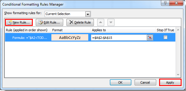
En primer lugar, seleccione su lista de fechas; en este ejemplo, las celdas A2:A15. En la pestaña Inicio, haga clic en Formato condicional > Administrar reglas. Consulte la siguiente captura de pantalla como guía:

Una vez que aparezca el cuadro de diálogo Usar formato condicional Administrar reglas, haga clic en el botón Nueva regla para crear una regla personalizada basada en fórmulas.

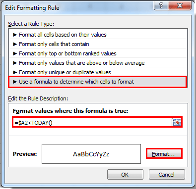
En el cuadro de diálogo Nueva regla de formato:
• Seleccione Usar una fórmula para determinar qué celdas dar formato. Esta opción le permite resaltar celdas de forma flexible según las fechas.
• Para resaltar fechas anteriores a hoy, copie y pegue la siguiente fórmula en el campo Dar formato a los valores donde esta fórmula sea verdadera:
=$A2<TODAY()• Para resaltar fechas posteriores a hoy (es decir, fechas futuras próximas), utilice esta fórmula:
=$A2>TODAY()• A continuación, haga clic en el botón Formato para definir el aspecto deseado (por ejemplo, cambiar el color de relleno o el estilo de fuente). Vea el ejemplo:
Especifique el formato deseado en el cuadro de diálogo Establecer formato de celda (por ejemplo, elija un color para que las fechas de vencimiento o futuras destaquen) y, a continuación, haga clic en Aceptar.
De vuelta en el cuadro de diálogo Usar formato condicional: Administrar reglas, verá su nueva lista de reglas. Para activar la regla, haga clic en Aplicar. Si desea configurar tanto el resaltado de fechas vencidas como de fechas futuras, repita los pasos para añadir una segunda regla utilizando la otra fórmula. Al volver nuevamente a Administrador de reglas, ambas reglas aparecerán ya listas.
Tras confirmar con Aceptar, su hoja de Excel distinguirá visualmente las fechas anteriores y posteriores a hoy, ofreciendo indicadores claros que impulsan la acción o la atención. Tanto las marcas de fechas vencidas como las próximas se actualizarán automáticamente conforme avancen los días, para que siempre tenga a simple vista los elementos más relevantes.

Este es el resultado: las fechas anteriores o posteriores a hoy están ahora resaltadas según su selección de formato, lo que simplifica la revisión y el seguimiento.

Consejos y advertencias: Asegúrese de que sus celdas de fecha estén formateadas como fechas (no como texto) para que las fórmulas funcionen correctamente. Si obtiene resultados inesperados, revise nuevamente el formato de fecha. En conjuntos de datos muy grandes, usar formato condicional puede afectar al rendimiento, por lo que conviene limitar siempre que sea posible el rango al que se aplica.
Resalte fechas anteriores a hoy o fechas futuras con KUTOOLS AI
Para usuarios que buscan una forma más sencilla e inteligente de resaltar fechas vencidas o futuras, KUTOOLS AI para Excel agiliza el proceso. En lugar de crear manualmente reglas con Formato condicional, basta con indicarle directamente a KUTOOLS AI, en lenguaje natural, lo que desea hacer. Este método es ideal si necesita resaltar fechas con frecuencia, pero quiere ahorrar tiempo, evitar configurar fórmulas o trabajar en entornos donde la precisión y la eficiencia son fundamentales.
Para utilizar KUTOOLS AI y resaltar fechas según su relación con la fecha actual:
- Haga clic en «Kutools» > «Asistente de IA» para abrir el panel «KUTOOLS AI Aide» y, a continuación, realice las siguientes operaciones:
- Seleccione el Rango de fechas que desee examinar.
- En el panel Asistente de IA, escriba un comando como:
— Para fechas vencidas:Resalte las fechas anteriores a hoy con color azul claro en el Seleccionar rango
— Para fechas futuras:Resalte las fechas posteriores a hoy con color azul claro en el Seleccionar rango - Pulse Intro o haga clic en Enviar. KUTOOLS AI analizará su solicitud. Una vez finalizado el procesamiento, haga clic en Ejecutar para aplicar automáticamente el formato.
KUTOOLS AI interpreta automáticamente su intención, seleccionando las fórmulas y formatos adecuados, lo que le ahorra tiempo y reduce errores manuales en la configuración. Este enfoque resulta especialmente útil en libros de trabajo dinámicos, para usuarios menos familiarizados con fórmulas o para quienes gestionan listas de fechas extensas y actualizadas con frecuencia.
Advertencia: KUTOOLS AI requiere conexión a Internet y tener instalada la versión más reciente de Kutools para Excel.
Marque y analice fechas con fórmulas de columnas auxiliares en Excel
En muchos casos reales, es posible que desee algo más que codificación por colores; por ejemplo, filtrar, ordenar o contar registros según si las fechas son anteriores o posteriores a hoy. El uso de columnas auxiliares con fórmulas de Excel le permite marcar claramente estos casos y aprovechar otras funciones de Excel (como filtros o tablas dinámicas) para realizar análisis en profundidad.
Ventajas: Fácil de configurar, compatible con ordenación y filtrado, y funciona en todas las versiones de Excel sin necesidad de permisos especiales.Inconvenientes: Requiere espacio adicional para columnas auxiliares; no ofrece coloreado directo salvo que se combine con formato condicional.
A continuación, se explica cómo utilizar una columna auxiliar para un análisis rápido de fechas:
1. Inserte una nueva columna junto a su lista de fechas (por ejemplo, la columna B al lado de las fechas en A2:A15).
2.En la celda B2 (suponiendo que A2 contiene su primera fecha), introduzca esta fórmula para marcar fechas vencidas:
=A2<TODAY()Esta fórmula devolverá VERDADERO si la fecha en A2 es anterior a hoy y FALSO en caso contrario.
3.Alternativamente, para marcar fechas futuras, utilice:
=A2>TODAY()4. Pulse Intro para confirmar la fórmula y, a continuación, arrastre el controlador hacia abajo para rellenar la columna en todas las filas que contengan fechas. Ahora podrá usar los resultados VERDADERO/FALSO para ordenar o filtrar registros según su estado de vencimiento o proximidad.
Si prefiere etiquetas de texto más claras, sustituya VERDADERO/FALSO por marcas más descriptivas. Por ejemplo:
=IF(A2<TODAY(),"Overdue",IF(A2>TODAY(),"Upcoming","Today"))Copie esta fórmula hacia abajo en todas las filas pertinentes según sea necesario. Puede filtrar, ordenar o utilizar la columna como criterio en otras funciones de Excel, como Usar formato condicional o tablas dinámicas. Este enfoque resulta especialmente útil para informes, paneles o la preparación de documentos impresos.
Nota: Si su columna de fechas no es la columna A, actualice la referencia de celda en la fórmula en consecuencia. Asegúrese de que el tipo de datos de las celdas de fecha esté configurado como fecha y no como texto para evitar resultados inconsistentes.
Artículos relacionados:
- ¿Cómo aplicar formato condicional a celdas según la primera letra o carácter en Excel?
- ¿Cómo aplicar formato condicional a celdas que contienen #N/A en Excel?
- ¿Cómo Formato condicional o resaltar la primera aparición en Excel?
- ¿Cómo Formato condicional porcentajes negativos en rojo en Excel?
Consejos rápidos para la resolución de problemas: Si el resaltado o las fórmulas no funcionan como se espera, verifique siempre el formato de las fechas y los rangos utilizados en las fórmulas. Use la Vista previa en «Usar formato condicional» para inspeccionar qué registros se ven afectados y compruebe cuidadosamente si hay reglas duplicadas que puedan solaparse o contradecirse entre sí. En tablas más grandes, las columnas auxiliares o las macros de VBA pueden agilizar el mantenimiento y ahorrar tiempo cuando se requieran actualizaciones frecuentes. Explore varios métodos para encontrar el flujo de trabajo que mejor se adapte a sus escenarios.
Las mejores herramientas de productividad para Office
Potencie sus habilidades en Excel con Kutools para Excel y experimente una eficiencia como nunca antes.Kutools para Excel ofrece más de 300 funciones avanzadas para aumentar su productividad y Ahorrar tiempo.Haga clic aquí para obtener la función que más necesita...
Office Tab aporta una interfaz con pestañas a Office y hace que su trabajo sea mucho más fácil
- Active la edición y lectura con pestañas en Word, Excel, PowerPoint, Publisher, Access, Visio y Project.
- Abra y cree varios documentos en nuevas pestañas dentro de la misma ventana, en lugar de hacerlo en ventanas separadas.
- ¡Aumente su productividad en un 50 % y elimine cientos de clics del ratón cada día!
Todos los complementos de Kutools en un solo instalador.
Kutools for Office es la suite que incluye complementos para Excel, Word, Outlook y PowerPoint, además de Office Tab Pro, ideal para equipos que trabajan en distintas aplicaciones de Office.
- Suite integral— complementos para Excel, Word, Outlook y PowerPoint + Office Tab Pro
- Un instalador, una licencia— configuración en minutos (compatible con MSI)
- Rendimiento mejorado en conjunto— productividad optimizada en todas las aplicaciones de Office
- Prueba gratuita de 30 días con todas las funciones— sin registro ni tarjeta de crédito
- La mejor relación calidad-precio— ahorre frente a la compra individual de complementos