¿Cómo buscar V y devolver múltiples valores correspondientes horizontalmente en Excel?

De forma predeterminada, la función BUSCARV puede devolver varios valores correspondientes en el nivel vertical en Excel; en algunos casos, es posible que desee devolver varios valores en el nivel horizontal como se muestra a continuación. Aquí te diré una fórmula que puede resolver esta tarea.
VLOOKUP y devuelve múltiples valores horizontalmente

VLOOKUP y devuelve múltiples valores horizontalmente

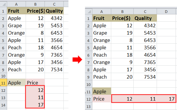
Por ejemplo, tiene un rango de datos como se muestra a continuación en la captura de pantalla y desea VLOOKUP los precios de Apple.

1. Seleccione una celda y escriba esta fórmula =INDEX($B$2:$B$9, SMALL(IF($A$11=$A$2:$A$9, ROW($A$2:$A$9)-ROW($A$2)+1), COLUMN(A1))) en él, y luego presione Mayús + Ctrl + Entrar y arrastre el controlador de autocompletar hacia la derecha para aplicar esta fórmula hasta #NUM! aparece. Ver captura de pantalla:

2. Luego borre el #NUM !. Ver captura de pantalla:

Consejo: En la fórmula anterior, B2: B9 es el rango de columna en el que desea devolver los valores, A2: A9 es el rango de columna en el que se encuentra el valor de búsqueda, A11 es el valor de búsqueda, A1 es la primera celda de su rango de datos , A2 es la primera celda del rango de columnas en el que se encuentra el valor de búsqueda.

Si desea devolver varios valores verticalmente, puede leer este artículo ¿Cómo buscar el valor devuelve múltiples valores correspondientes en Excel?

Combine fácilmente varias hojas / libro de trabajo en una sola hoja o libro de trabajo

Combinar varias hojas o libros de trabajo en una sola hoja o libro de trabajo puede ser complicado en Excel, pero con la Combinar función en Kutools para Excel, puede combinar fusionar docenas de hojas / libros de trabajo en una hoja o libro de trabajo, también, puede consolidar las hojas en una por varios clics solamente.  ¡Haga clic para obtener una prueba gratuita de 30 días con todas las funciones!

Kutools para Excel: con más de 300 prácticos complementos de Excel, prueba gratis sin límite en 30 días.

Las mejores herramientas de productividad de oficina

🤖	Asistente de IA de Kutools: Revolucionar el análisis de datos basado en: Ejecución inteligente   |  Generar codigo  |  Crear fórmulas personalizadas  |  Analizar datos y generar gráficos  |  Invocar funciones de Kutools...
	Características populares: Buscar, resaltar o identificar duplicados   |  Eliminar filas en blanco   |  Combine columnas o celdas sin perder datos   |   Ronda sin fórmula ...
	Super búsqueda: Búsqueda virtual de criterios múltiples  |   Búsqueda V de valores múltiples  |   VLookup en varias hojas   |   Búsqueda difusa ....
	Lista desplegable avanzada: Crear rápidamente una lista desplegable   |  Lista desplegable dependiente   |  Lista desplegable de selección múltiple ....
	Administrador de columnas: Agregar un número específico de columnas  |  Mover columnas  |  Toggle Estado de visibilidad de columnas ocultas  |  Comparar rangos y columnas ...
	Características destacadas: Enfoque de cuadrícula   |  Vista de diseño   |   Gran barra de fórmulas   |  Administrador de hojas y libros de trabajo   |  Biblioteca de Recursos (Texto automático)   |  Selector de fechas   |  Combinar hojas de trabajo   |  Cifrar/descifrar celdas   |  Enviar correos electrónicos por lista   |  Súper filtro   |   Filtro especial (filtro negrita/cursiva/tachado...) ...
	Los 15 mejores conjuntos de herramientas:  12 Texto Herramientas (Añadir texto, Quitar caracteres, ...)   |   50+ Tabla Tipos (Diagrama de Gantt, ...)   |   40+ Práctico Fórmulas (Calcular la edad según el cumpleaños, ...)   |   19 Inserción Herramientas (Insertar código QR, Insertar imagen desde la ruta, ...)   |   12 Conversión Herramientas (Números a palabras, Conversión de Moneda, ...)   |   7 Fusionar y dividir Herramientas (Filas combinadas avanzadas, Células partidas, ...)   |   ... y más

Mejore sus habilidades de Excel con Kutools for Excel y experimente la eficiencia como nunca antes. Kutools for Excel ofrece más de 300 funciones avanzadas para aumentar la productividad y ahorrar tiempo.  Haga clic aquí para obtener la función que más necesita...

Leer más ... Descarga gratis...

---

Office Tab lleva la interfaz con pestañas a Office y hace que su trabajo sea mucho más fácil

• Habilite la edición y lectura con pestañas en Word, Excel, PowerPoint, Publisher, Access, Visio y Project.
• Abra y cree varios documentos en nuevas pestañas de la misma ventana, en lugar de en nuevas ventanas.
• ¡Aumenta su productividad en un 50% y reduce cientos de clics del mouse todos los días!

Leer más ... Descarga gratis...