¿Cómo encontrar el primer o último viernes de cada mes en Excel?
Normalmente, el viernes es el último día laborable del mes. ¿Cómo puede encontrar el primer o último viernes en función de una fecha dada en Excel? En este artículo, le guiaremos paso a paso para utilizar dos fórmulas sencillas y precisas que le permitirán hallar el primer o último viernes de cada mes.
Encontrar el primer viernes de un mes
Encontrar el último viernes de un mes
Encontrar el primer viernes de un mes
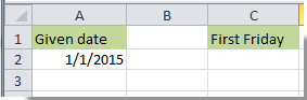
Por ejemplo, supongamos que la fecha 1/1/2015 se encuentra en la celda A2, tal como se muestra en la siguiente captura de pantalla. Si desea determinar el primer viernes del mes a partir de dicha fecha, siga estos pasos.
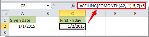
1. Seleccione una celda para mostrar el resultado; en este caso, elegimos la celda C2.
2. Copie y pegue la siguiente fórmula en ella y, a continuación, pulse la tecla Entrar.
=CEILING(EOMONTH(A2,-1)-5,7)+6
Notas:
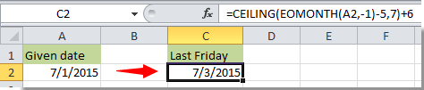
Encontrar el último viernes de un mes
La fecha indicada, 1/1/2015, se encuentra en la celda A2. Para hallar el último viernes de ese mes en Excel, siga estos sencillos pasos.
1. Seleccione una celda, copie la siguiente fórmula en ella y pulse Entrar para obtener el resultado.
=DATE(YEAR(A2),MONTH(A2)+1,0)+MOD(-WEEKDAY(DATE(YEAR(A2),MONTH(A2)+1,0),2)-2,-7)

Nota: Puede sustituir A2 en la fórmula por la celda que contenga su fecha.
Artículos relacionados:
- ¿Cómo encontrar los 5 valores más bajos y más altos en una lista en Excel?
- ¿Cómo puedo saber si un libro de trabajo específico está abierto en Excel?
- ¿Cómo puedo saber si una celda está referenciada en otra celda de Excel?
- ¿Cómo encontrar la fecha más cercana a hoy en una lista de Excel?
Las mejores herramientas de productividad para Office
Potencie sus habilidades en Excel con Kutools para Excel y experimente una eficiencia como nunca antes.Kutools para Excel ofrece más de 300 funciones avanzadas para aumentar su productividad y Ahorrar tiempo.Haga clic aquí para obtener la función que más necesita...
Office Tab aporta una interfaz con pestañas a Office y hace que su trabajo sea mucho más fácil
- Active la edición y lectura con pestañas en Word, Excel, PowerPoint, Publisher, Access, Visio y Project.
- Abra y cree varios documentos en nuevas pestañas dentro de la misma ventana, en lugar de hacerlo en ventanas separadas.
- ¡Aumente su productividad en un 50 % y elimine cientos de clics del ratón cada día!
Todos los complementos de Kutools en un solo instalador.
Kutools for Office es la suite que incluye complementos para Excel, Word, Outlook y PowerPoint, además de Office Tab Pro, ideal para equipos que trabajan en distintas aplicaciones de Office.
- Suite integral— complementos para Excel, Word, Outlook y PowerPoint + Office Tab Pro
- Un instalador, una licencia— configuración en minutos (compatible con MSI)
- Rendimiento mejorado en conjunto— productividad optimizada en todas las aplicaciones de Office
- Prueba gratuita de 30 días con todas las funciones— sin registro ni tarjeta de crédito
- La mejor relación calidad-precio— ahorre frente a la compra individual de complementos