Saltar al contenido principal

¿Cómo buscar con vlookup el primer, segundo o enésimo valor de coincidencia en Excel?

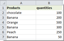
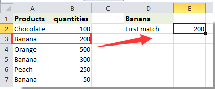
Supongamos que tiene dos columnas con Productos y cantidades como se muestra a continuación. Para averiguar rápidamente las cantidades del primer o segundo plátano, ¿qué harías?

Aquí, la función vlookup puede ayudarlo a lidiar con este problema. En este artículo, le mostraremos cómo buscar con vlookup el primer, segundo o n-ésimo valor de coincidencia con la función Vlookup en Excel.

Vlookup encuentra el primer, segundo o enésimo valor de coincidencia en Excel con fórmula

Vlookup encuentra fácilmente el primer valor de coincidencia en Excel con Kutools para Excel


Vlookup encuentra el primer, segundo o enésimo valor de coincidencia en Excel

Haga lo siguiente para encontrar el primer, segundo o enésimo valor de coincidencia en Excel.

1. En la celda D1, ingrese los criterios que desea visualizar, aquí ingrese Banana.

2. Aquí encontraremos el primer valor de coincidencia de banana. Seleccione una celda en blanco como E2, copie y pegue la fórmula =INDEX($B$2:$B$6,MATCH(TRUE,EXACT($D$1,$A$2:$A$6),0)) en la barra de fórmulas y luego presione Ctrl + Shift + Participar llaves al mismo tiempo

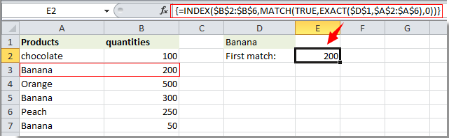
Note: En esta fórmula, $ B $ 2: $ B $ 6 es el rango de los valores coincidentes; $ A $ 2: $ A $ 6 es el rango con todos los criterios para vlookup; $ D $ 1 es la celda que contiene los criterios de vlookup especificados.

Luego, obtendrá el primer valor de coincidencia de banana en la celda E2. Con esta fórmula, solo puede obtener el primer valor correspondiente según sus criterios.

Para obtener cualquier enésimo valor relativo, puede aplicar la siguiente fórmula: =INDEX($B$2:$B$6,SMALL(IF($D$1=$A$2:$A$6,ROW($A$2:$A$6)-ROW($A$2)+1),1)) + Ctrl + Shift + Participar claves juntas, esta fórmula devolverá el primer valor coincidente.

Notas:

1. Para encontrar el segundo valor de coincidencia, cambie la fórmula anterior a =INDEX($B$2:$B$6,SMALL(IF($D$1=$A$2:$A$6,ROW($A$2:$A$6)-ROW($A$2)+1),2))y luego presione Ctrl + Shift + Participar teclas simultáneamente. Ver captura de pantalla:

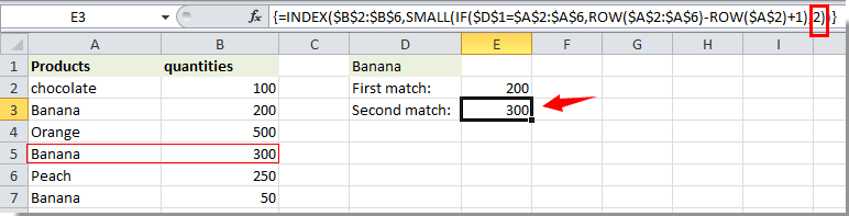
2. El último número en la fórmula anterior significa el enésimo valor de coincidencia de los criterios de vlookup. Si lo cambia a 3, obtendrá el tercer valor de coincidencia y, si cambia an, se encontrará el enésimo valor de coincidencia.


Vlookup encuentra el primer valor de coincidencia en Excel con Kutools para Excel

YPuede encontrar fácilmente el primer valor de coincidencia en Excel sin recordar fórmulas con el Busque un valor en la lista fórmula fórmula de Kutools for Excel.

Antes de aplicar Kutools for Excel, Por favor descargarlo e instalarlo en primer lugar.

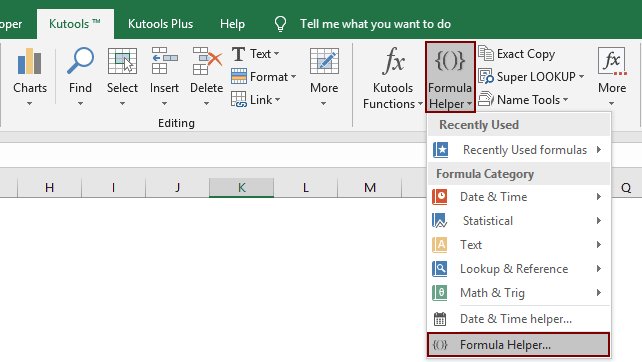
1. Seleccione una celda para ubicar el primer valor coincidente (dice celda E2) y luego haga clic en Kutools > Ayudante de fórmula > Ayudante de fórmula. Ver captura de pantalla:

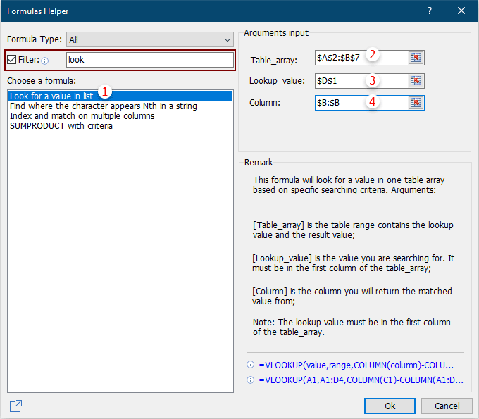
3. En el Ayudante de fórmula cuadro de diálogo, configure de la siguiente manera:

  • 3.1 En el Elige una fórmula cuadro, busque y seleccione Busque un valor en la lista;
    Tips: Puede comprobar el Filtrar cuadro, ingrese cierta palabra en el cuadro de texto para filtrar la fórmula rápidamente.
  • 3.2 En el Matriz de tabla cuadro, seleccione el tabla que contiene los primeros valores coincidentes.;
  • 3.2 En el Valor de búsqueda cuadro, seleccione la celda que contiene el criterios devolverá el primer valor basado en;
  • 3.3 En el Columna , especifique la columna de la que devolverá el valor coincidente. O puede ingresar el número de columna en el cuadro de texto directamente según lo necesite.
  • 3.4 Haga clic en OK botón. Ver captura de pantalla:

Ahora el valor de celda correspondiente se completará automáticamente en la celda C10 según la selección de la lista desplegable.

  Si desea tener una prueba gratuita (30 días) de esta utilidad, haga clic para descargarloy luego vaya a aplicar la operación según los pasos anteriores.

Las mejores herramientas de productividad de oficina

🤖 Asistente de IA de Kutools: Revolucionar el análisis de datos basado en: Ejecución inteligente   |  Generar codigo  |  Crear fórmulas personalizadas  |  Analizar datos y generar gráficos  |  Invocar funciones de Kutools...
Características populares: Buscar, resaltar o identificar duplicados   |  Eliminar filas en blanco   |  Combine columnas o celdas sin perder datos   |   Ronda sin fórmula ...
Super búsqueda: Búsqueda virtual de criterios múltiples    Búsqueda V de valores múltiples  |   VLookup en varias hojas   |   Búsqueda difusa ....
Lista desplegable avanzada: Crear rápidamente una lista desplegable   |  Lista desplegable dependiente   |  Lista desplegable de selección múltiple ....
Administrador de columnas: Agregar un número específico de columnas  |  Mover columnas  |  Toggle Estado de visibilidad de columnas ocultas  |  Comparar rangos y columnas ...
Características destacadas: Enfoque de cuadrícula   |  Vista de diseño   |   Gran barra de fórmulas    Administrador de hojas y libros de trabajo   |  Biblioteca de Recursos (Texto automático)   |  Selector de fechas   |  Combinar hojas de trabajo   |  Cifrar/descifrar celdas    Enviar correos electrónicos por lista   |  Súper filtro   |   Filtro especial (filtro negrita/cursiva/tachado...) ...
Los 15 mejores conjuntos de herramientas12 Texto Herramientas (Añadir texto, Quitar caracteres, ...)   |   50+ Tabla Tipos (Diagrama de Gantt, ...)   |   40+ Práctico Fórmulas (Calcular la edad según el cumpleaños, ...)   |   19 Inserción Herramientas (Insertar código QR, Insertar imagen desde la ruta, ...)   |   12 Conversión Herramientas (Números a palabras, Conversión de Moneda, ...)   |   7 Fusionar y dividir Herramientas (Filas combinadas avanzadas, Células partidas, ...)   |   ... y más

Mejore sus habilidades de Excel con Kutools for Excel y experimente la eficiencia como nunca antes. Kutools for Excel ofrece más de 300 funciones avanzadas para aumentar la productividad y ahorrar tiempo.  Haga clic aquí para obtener la función que más necesita...

Descripción


Office Tab lleva la interfaz con pestañas a Office y hace que su trabajo sea mucho más fácil

  • Habilite la edición y lectura con pestañas en Word, Excel, PowerPoint, Publisher, Access, Visio y Project.
  • Abra y cree varios documentos en nuevas pestañas de la misma ventana, en lugar de en nuevas ventanas.
  • ¡Aumenta su productividad en un 50% y reduce cientos de clics del mouse todos los días!
Comments (43)
No ratings yet. Be the first to rate!
This comment was minimized by the moderator on the site
You only return first match with VLOOKUP so your article "How To Vlookup Find The First, 2nd Or Nth Match Value In Excel?" does not make any sense....
This comment was minimized by the moderator on the site
Hi Sima,
"VLOOKUP" is a Google search term, so I used it as a keyword for the article title. The main operation of this article is to lookup values. I'm sorry for the misunderstanding.
This comment was minimized by the moderator on the site
What if the next record on col b is a duplicate how do ignore duplicate? Let's Banana has quantities of 200 twice? Can you please help me figure out how to ignore the duplicate?
This comment was minimized by the moderator on the site
Cna anybody Explain the small function with the IF statement for me please? I don't really understand how that array works :(
This comment was minimized by the moderator on the site
The following formulas works perfect for me:
(a) or(b) =IF(H8='Raw Data'!B4,INDEX('Raw Data'!H6:H20,SMALL(IF(C18='Raw Data'!B6:B20,ROW('Raw Data'!B6:B20)-ROW('Raw Data'!B6:B20)+1),1)))

However, I have encountered a problem where there are 7 sets of the same criteria but in different columns:(1) can the above formula (a) be repeated and search in a different cells in a single formula and(2) the above formula (b) only allows up to two sets of the similar search with matched value result but when trying for the third set in the formula as showed below, Microsoft Excel appeared as "You've entered too many arguments for this function."
=<span style="letter-spacing: 0.2px; color: inherit; font-family: inherit; font-style: inherit; font-variant-ligatures: inherit; font-variant-caps: inherit; font-weight: inherit;">IF(H8='Raw Data'!J4,INDEX('Raw Data'!P6:P20,SMALL(IF(C18='Raw Data'!J6:J20,ROW('Raw Data'!J6:J20)-ROW('Raw Data'!J6:J20)+1),1))),</span>
This comment was minimized by the moderator on the site
What do Ctrl + Shift + Enter do?? At the beginning I didn'
This comment was minimized by the moderator on the site
Hi,An array formula needs to hit the Ctrl + Shift + Enter keys simultaneously to get the correct result.
This comment was minimized by the moderator on the site
I have a scenario... How do I get last price of anything for reference... Example: Banana first price was 200... While purchasing for second time; I need to display 200 in my expected price cell and then if I buy that on the day at 220, I will put this value manually as 220... Whenever next time I will buy banana; I need to display 220 from the last purchase price
This comment was minimized by the moderator on the site
Try =INDEX($B$2:$B$6,XMATCH(TRUE,EXACT($D$1,$A$2:$A$6),0,-1))

This is essentially reversing the search order and returning the first match using the XMATCH function.

Better late than never, hopefully helps someone :)
This comment was minimized by the moderator on the site
Perfect explanation, thanks.
This comment was minimized by the moderator on the site
If the first or any of the other entry's for 'banana' column B was blank cell, of which I don't require this number, what changes are required to this formula to skip blank cell in column B.
This comment was minimized by the moderator on the site
Sorry I am using this formula
=INDEX($B$2:$B$6,SMALL(IF($D$1=$A$2:$A$6,ROW($A$2:$A$6)-ROW($A$2)+1),1))
This comment was minimized by the moderator on the site
SOLVED:
=SMALL(IF(A2:A7=D1,IF(B2:B7<>"",B2:B7)),1)

If 2nd or 3rd number required exchange ),1) to 2 or 3

This formula does not require index, as it directly looks at the value in Cell
This comment was minimized by the moderator on the site
Correction to previous formula:
The value was reading either the lesser or greater.

Updated formula
=INDEX($B$2:$B$7,SMALL(IF($A2:$A6=$D$1,IF($B$2:$B$7<>"",ROW($A2:$A6)-ROW($A2)+1)),1))

This skips blank cell and places value of non blank cell. Replace +1 with +2 or +3 for 2nd or 3rd value
This comment was minimized by the moderator on the site
And if you want the last, second last, nth last just add a counter (count the number of events already hapenned) to the end and subtract it by 0,1,n respectively.

Thank you so much! I was searching for this for a long time
This comment was minimized by the moderator on the site
Good Day,
Sorry can't help you with this yet. Thank you for your comment.
This comment was minimized by the moderator on the site
Is it possible to find an average of the non-unique data. Or would it be possible to have a list dropdown on the cell of the various values?
This comment was minimized by the moderator on the site
Good Day,
Sorry can't help you with this yet. Thank you for your comment.
There are no comments posted here yet
Load More
Please leave your comments in English
Posting as Guest
×
Rate this post:
0   Characters
Suggested Locations