¿Cómo concatenar celdas cuando hay un valor coincidente en otra columna de Excel?
Como se muestra en la siguiente captura de pantalla, si desea concatenar las celdas de la segunda columna según los valores idénticos de la primera, dispone de varios métodos. En este artículo, le presentamos tres formas eficaces de lograrlo.

Concatenar celdas si hay valores iguales con fórmulas y filtro
Las siguientes fórmulas permiten concatenar las celdas de una columna según los valores coincidentes en otra columna.
1. Seleccione una celda vacía junto a la segunda columna (aquí seleccionamos la celda C2), introduzca la fórmula =IF(A2<>A1,B2,C1 & "," & B2) en la Barra de fórmulas y pulse la tecla Entrar.

2. A continuación, seleccione la celda C2 y arrastre el controlador de relleno hasta las celdas que desee combinar.

3. Introduzca la fórmula =IF(A2<>A3,CONCATENATE(A2,«»",C2,"«»«),»") en la celda D2 y arrastre el controlador de relleno al resto de las celdas.

4. Seleccione la celda D1 y haga clic en Datos > Filtro. Vea la captura de pantalla:

5. Haga clic en la flecha desplegable de la celda D1, desactive la casilla (Vacías) y, a continuación, haga clic en el botón Aceptar.

Podrá comprobar que las celdas se han concatenado cuando los valores de la primera columna coincidan.

Nota: Para utilizar correctamente las fórmulas anteriores, los valores iguales en la columna A deben estar contiguos.
Concatene fácilmente celdas si hay valores iguales con Kutools para Excel (solo unos pocos clics)
El método descrito anteriormente requiere crear dos columnas auxiliares e implica varios pasos, lo que puede resultar incómodo. Si busca una forma más sencilla, considere utilizar la herramienta Combinar filas avanzado de Kutools para Excel. Con solo unos pocos clics, esta utilidad le permite concatenar celdas con un delimitador específico, haciendo que el proceso sea rápido y sin complicaciones.
1. Haga clic en Kutools > Combinar y dividir > Combinar filas avanzado para activar esta función.
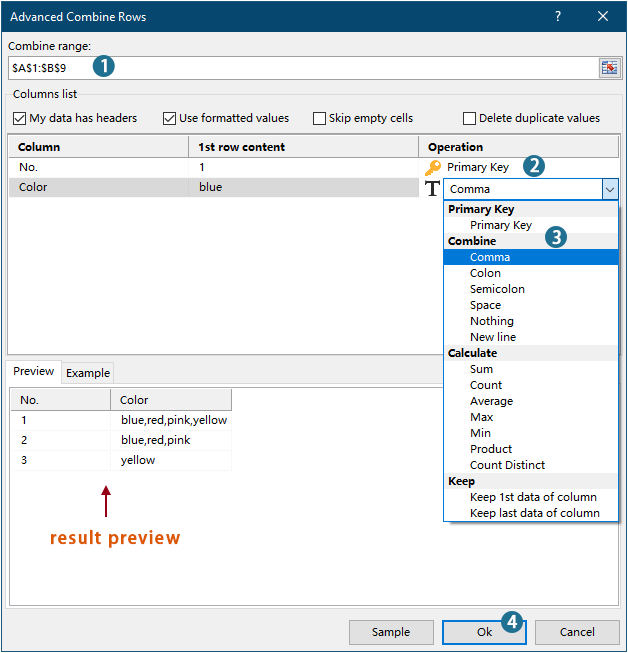
2. En el cuadro de diálogo Combinar filas avanzado, solo tiene que:
- Seleccione el rango que desea concatenar;
- Establezca como columna de clave principal la columna que contenga los mismos valores.
- Separador para combinar celdas.
- Haga clic en Aceptar.
Resultado

Kutools para Excel: potencie Excel con más de 300 herramientas esenciales, agilice y simplifique su trabajo, y aproveche las funciones de IA para un procesamiento de datos más inteligente y una mayor productividad.Consígalo ahora
- Para obtener más información sobre esta función, consulte este artículo:Combine rápidamente valores iguales o Fila duplicada en Excel
Concatenar celdas si hay valores iguales con código VBA
También puede usar código VBA para concatenar celdas en una columna cuando haya un valor coincidente en otra columna.
1. Pulse las teclas Alt + F11 para abrir la ventana de Microsoft Visual Basic para Aplicaciones.
2. En la ventana de Microsoft Visual Basic para Aplicaciones, haga clic en Insertar > Módulo. A continuación, copie y pegue el siguiente código en la ventana del Módulo.
Código VBA: concatenar celdas si hay valores iguales
Sub ConcatenateCellsIfSameValues()
	Dim xCol As New Collection
	Dim xSrc As Variant
	Dim xRes() As Variant
	Dim I As Long
	Dim J As Long
	Dim xRg As Range
	xSrc    = Range("A1", Cells(Rows.Count, "A").End(xlUp)).Resize(, 2)
	Set xRg = Range("D1")
	On Error Resume Next
	For I = 2 To UBound(xSrc)
		xCol.Add xSrc(I, 1), TypeName(xSrc(I, 1)) & CStr(xSrc(I, 1))
	Next I
	On Error GoTo 0
	ReDim xRes(1 To xCol.Count + 1, 1 To 2)
	xRes(1, 1) = "No"
	xRes(1, 2) = "Combined Color"
	For I = 1 To xCol.Count
		xRes(I + 1, 1) = xCol(I)
		For J = 2 To UBound(xSrc)
			If xSrc(J, 1) = xRes(I + 1, 1) Then
				xRes(I + 1, 2) = xRes(I + 1, 2) & ", " & xSrc(J, 2)
			End If
		Next J
		xRes(I + 1, 2) = Mid(xRes(I + 1, 2), 2)
	Next I
	Set xRg = xRg.Resize(UBound(xRes, 1), UBound(xRes, 2))
	xRg.NumberFormat = "@"
	xRg = xRes
	xRg.EntireColumn.AutoFit
End SubNotas:
3. Pulse la tecla F5 para ejecutar el código y obtener así los resultados concatenados en un rango limitado.

Demostración: Concatene fácilmente celdas si hay valores iguales con Kutools para Excel
Las mejores herramientas de productividad para Office
Potencie sus habilidades en Excel con Kutools para Excel y experimente una eficiencia como nunca antes.Kutools para Excel ofrece más de 300 funciones avanzadas para aumentar su productividad y Ahorrar tiempo.Haga clic aquí para obtener la función que más necesita...
Office Tab aporta una interfaz con pestañas a Office y hace que su trabajo sea mucho más fácil
- Active la edición y lectura con pestañas en Word, Excel, PowerPoint, Publisher, Access, Visio y Project.
- Abra y cree varios documentos en nuevas pestañas dentro de la misma ventana, en lugar de hacerlo en ventanas separadas.
- ¡Aumente su productividad en un 50 % y elimine cientos de clics del ratón cada día!
Todos los complementos de Kutools en un solo instalador.
Kutools for Office es la suite que incluye complementos para Excel, Word, Outlook y PowerPoint, además de Office Tab Pro, ideal para equipos que trabajan en distintas aplicaciones de Office.
- Suite integral— complementos para Excel, Word, Outlook y PowerPoint + Office Tab Pro
- Un instalador, una licencia— configuración en minutos (compatible con MSI)
- Rendimiento mejorado en conjunto— productividad optimizada en todas las aplicaciones de Office
- Prueba gratuita de 30 días con todas las funciones— sin registro ni tarjeta de crédito
- La mejor relación calidad-precio— ahorre frente a la compra individual de complementos