¿Cómo buscarV y concatenar varios valores coincidentes en Excel?
Al usar BUSCARV en Excel, la función normalmente devuelve solo la primera coincidencia que encuentra para un criterio dado. Sin embargo, en muchos escenarios habituales es necesario recuperar y combinar todos los valores asociados a una clave específica, como listar a todos los alumnos de una clase o todos los productos de una categoría. Debido a esta limitación de BUSCARV estándar, es natural preguntarse cómo combinar varias coincidencias en una sola celda. A continuación, exploraremos varios métodos prácticos y eficaces para lograrlo, adaptados a distintas versiones de Excel y preferencias de usuario.
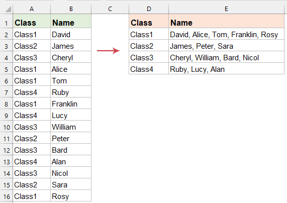
BuscarV y concatenar varios valores correspondientes en Excel
BuscarV y concatenar varios valores correspondientes con las funciones TEXTJOIN y FILTRO
Si utiliza Excel 365 o Excel 2021, la combinación de las funciones TEXTJOIN y FILTRO ofrece un enfoque eficaz basado en fórmulas para buscar y concatenar todas las coincidencias. Esta solución es ideal para conjuntos de datos dinámicos y actualizados, ya que refresca automáticamente los resultados cuando cambian los datos de origen. Se recomienda especialmente si su versión de Excel incluye la función FILTRO, disponible exclusivamente en versiones recientes de Office.
En la celda de destino, introduzca la siguiente fórmula y arrástrela hacia abajo para aplicarla a otras filas. Todos los valores coincidentes se extraerán y combinarán en una sola celda. Vea la captura de pantalla:
=TEXTJOIN(", ", TRUE, FILTER($B$2:$B$16, $A$2:$A$16=D2, ""))
- FILTER($B$2:$B$16, $A$2:$A$16=D2, «»)Esta parte de la fórmula evalúa cada valor del rango $A$2:$A$16; si coincide con el valor de D2, incluye el valor correspondiente del rango $B$2:$B$16 en la matriz de resultados.
- $B$2:$B$16El rango del que se extraerán los valores coincidentes.
- $A$2:$A$16=D2La condición que determina qué valores se seleccionan; únicamente se procesarán las filas en las que el rango $A$2:$A$16 coincida con el contenido de D2.
- TEXTJOIN(", ", VERDADERO, ...): Esta función toma la salida de la función FILTRO (una matriz de coincidencias) y las concatena en una sola cadena de texto, separadas por el delimitador especificado (coma y espacio), ignorando automáticamente las entradas vacías.
- ",": Establece la coma seguida de un espacio como separador; puedes cambiar este símbolo según tus necesidades, por ejemplo, usar punto y coma o saltos de línea.
- VERDADERO: Garantiza que las celdas vacías se omitan en el proceso de combinación, obteniendo así un resultado con formato limpio.
Nota especial: Este método requiere Excel 365 o Excel 2021 y no es compatible con versiones anteriores (por ejemplo, Excel 2019, 2016 o versiones más antiguas). ¡Asegúrese siempre de comprobar su versión de Excel antes de aplicarlo!
Consejo: Si su valor de búsqueda (por ejemplo, D2) cambia o se añaden nuevos elementos coincidentes en el rango de datos, el resultado se actualiza automáticamente sin necesidad de realizar pasos adicionales.
Limitaciones potenciales: En conjuntos de datos muy grandes, el tiempo de cálculo de la fórmula puede aumentar. Asimismo, los usuarios deben asegurarse de que no haya celdas combinadas en los rangos de búsqueda o resultado, ya que podrían provocar errores en la fórmula.
BuscarV y concatenar varios valores correspondientes con Kutools para Excel
Si los métodos basados en fórmulas integradas le resultan complicados o su versión de Excel no admite funciones avanzadas como TEXTJOIN y FILTRO, Kutools para Excel le ofrece una solución gráfica fácil de usar. La función Búsqueda uno a muchos de Kutools le permite buscar y concatenar varios resultados coincidentes en pocos pasos, ideal tanto para principiantes como para usuarios avanzados. Con Kutools, no necesita escribir fórmulas ni códigos complejos, y resulta especialmente útil al trabajar con conjuntos de datos grandes o variables que requieren búsquedas y agregaciones repetidas.
Tras instalar Kutools para Excel, siga los pasos siguientes:
Haga clic en Kutools > Super BUSCARV > Búsqueda uno a muchos (devolver múltiples resultados) para abrir el cuadro de diálogo de configuración. En este cuadro podrá configurar rápidamente la búsqueda y los ajustes de salida siguiendo estos pasos:
- Seleccione las celdas de destino para los resultados concatenados y las celdas que contienen los valores que desea buscar;
- Indique el rango de la tabla que contiene tanto la columna de claves de búsqueda como la de resultados;
- Especifique qué columna contiene las claves de búsqueda (Columna clave) y qué columna contiene los valores que se concatenarán (Columna de devolución);
- Haga clic en el botón Aceptar para confirmar la configuración y procesar los datos.


Resultado: Kutools mostrará ahora todos los valores coincidentes concatenados en la celda de salida seleccionada. Consulte la captura de pantalla:
Este método es ideal para quienes prefieren trabajar directamente desde la interfaz de Excel, sin necesidad de recurrir a fórmulas o códigos complejos. Además, minimiza el riesgo de errores en las fórmulas y potencia la productividad al gestionar tareas repetitivas de búsqueda y concatenación.
BuscarV y concatenar varios valores correspondientes con una función definida por el usuario
Para usuarios con experiencia en VBA (Visual Basic para Aplicaciones) o que utilicen versiones antiguas de Excel sin funciones de matrices dinámicas ni la función FILTRO, es posible crear una función personalizada (UDF) que permita una concatenación flexible de múltiples resultados. Este método es compatible con todas las versiones de Excel y se puede adaptar a distintos separadores o condiciones específicas.
1. Mantenga pulsadas las teclas ALT + F11 para abrir la ventana de Microsoft Visual Basic para Aplicaciones.
2. Haga clic en Insertar > Módulo y pegue el siguiente código en la ventana del módulo.
Código VBA: BuscarV y concatenar varios valores coincidentes en una celda
Function ConcatenateMatches(LookupValue As String, LookupRange As Range, ReturnRange As Range, Optional Delimiter As String = ", ") As String
'Updateby Extendoffice
    Dim Cell As Range
    Dim Result As String
    Result = ""
    For Each Cell In LookupRange
        If Cell.Value = LookupValue Then
            Result = Result & Cell.Offset(0, ReturnRange.Column - LookupRange.Column).Value & Delimiter
        End If
    Next Cell
    If Result <> "" Then
        Result = Left(Result, Len(Result) - Len(Delimiter))
    End If
    ConcatenateMatches = Result
End Function
3. Guarde y cierre el editor de VBA. Vuelva a su hoja de cálculo e introduzca esta UDF escribiendo la fórmula: =ConcatenateMatches(D2, $A$2:$A$16, $B$2:$B$16) en una celda vacía donde desee ver el resultado. Arrastre el controlador de relleno hacia abajo para aplicar la fórmula a otras celdas según sea necesario. Todos los valores que coincidan con un valor de búsqueda específico se devolverán y concatenarán en una sola celda, separados por una coma y un espacio. Vea la captura de pantalla:

- D2: El valor que se busca encontrar en su conjunto de datos (ValorBuscado).
- A2:A16: El rango en el que la función busca el valor de búsqueda (RangoBúsqueda).
- B2:B16: El rango que contiene los valores que se concatenarán cuando coincida el valor de búsqueda (RangoResultado).
BuscarV y concatenar varios valores correspondientes con código VBA
Para escenarios que requieran uso repetido o para quienes prefieran evitar funciones personalizadas en las celdas de la hoja de cálculo, puede utilizar una macro VBA lista para concatenar resultados directamente. Este método es ideal en entornos compartidos donde no todos los usuarios cuenten con la misma versión del software o con los mismos complementos instalados.
1. Haga clic en Herramientas para desarrolladores > Visual Basic para abrir el editor de VBA.
2. En la ventana de VBA, haga clic en Insertar > Módulo y luego pegue este código en el módulo:
Sub VLookupAndConcatenate()
    Dim ws As Worksheet
    Dim dataRange As Range, lookupRange As Range, resultRange As Range
    Dim dict As Object
    Dim i As Long, lastRow As Long
    Dim lookupValue As Variant, result As String
    Dim delimiter As String
    delimiter = ", "
    Set dict = CreateObject("Scripting.Dictionary")
    Set ws = ActiveSheet
    On Error Resume Next
    Set dataRange = Application.InputBox( _
        Prompt:="Please select the data range (contains lookup column and result column)", _
        Title:="Select Data Range", _
        Type:=8)
    On Error GoTo 0
    If dataRange Is Nothing Then Exit Sub
    On Error Resume Next
    Set lookupRange = Application.InputBox( _
        Prompt:="Please select the lookup range (single column)", _
        Title:="Select Lookup Range", _
        Type:=8)
    On Error GoTo 0
    If lookupRange Is Nothing Then Exit Sub
    On Error Resume Next
    Set resultRange = Application.InputBox( _
        Prompt:="Please select the starting cell for results output", _
        Title:="Select Output Location", _
        Type:=8)
    On Error GoTo 0
    If resultRange Is Nothing Then Exit Sub
    resultRange.Resize(lookupRange.Rows.Count, 1).ClearContents
    For i = 1 To dataRange.Rows.Count
        lookupValue = dataRange.Cells(i, 1).Value
        If Not dict.Exists(lookupValue) Then
            dict.Add lookupValue, dataRange.Cells(i, 2).Value
        Else
            dict(lookupValue) = dict(lookupValue) & delimiter & dataRange.Cells(i, 2).Value
        End If
    Next i
    For i = 1 To lookupRange.Rows.Count
        lookupValue = lookupRange.Cells(i, 1).Value
        If dict.Exists(lookupValue) Then
            resultRange.Cells(i, 1).Value = dict(lookupValue)
        Else
            resultRange.Cells(i, 1).Value = "Not Found"
        End If
    Next i
    MsgBox "Operation completed! Processed " & lookupRange.Rows.Count & " lookup values.", vbInformation
End Sub
3. Haga clic en el botón ![]() para ejecutar la macro. A continuación, aparecerán cuadros de diálogo que le pedirán que seleccione su rango de datos, rango de búsqueda y rango de resultados. El resultado concatenado se mostrará directamente en las celdas de salida seleccionadas.
para ejecutar la macro. A continuación, aparecerán cuadros de diálogo que le pedirán que seleccione su rango de datos, rango de búsqueda y rango de resultados. El resultado concatenado se mostrará directamente en las celdas de salida seleccionadas.
Este enfoque mediante macro resulta especialmente útil si realiza con frecuencia búsquedas de concatenación múltiple con valores diferentes, ya que evita saturar la hoja de cálculo con llamadas a funciones personalizadas.
Puede ajustar fácilmente el delimitador en el código si es necesario y ampliar la macro para exportar los resultados a una celda o archivo, según su flujo de trabajo.
Es posible concatenar varios valores correspondientes en Excel mediante diversos enfoques, cada uno con ventajas específicas según su situación. Ya sea que elija fórmulas de matrices dinámicas, complementos como Kutools para Excel o métodos basados en VBA, potenciará su capacidad para analizar y presentar datos agrupados de forma eficiente. En función del tamaño y la complejidad de su conjunto de datos, considere qué enfoque ofrece el mejor rendimiento y la mayor facilidad de mantenimiento para usted o su equipo. En las operaciones diarias, verifique la coherencia de los datos, evite Combinada y confirme los rangos de referencia para obtener resultados óptimos. Si detecta errores en los cálculos de fórmulas, revise cuidadosamente que sus rangos coincidan con los datos y que esté utilizando el método adecuado de introducción de fórmulas para su versión de Excel.
Para dominar técnicas avanzadas de Excel y acceder a una amplia variedad de guías prácticas paso a paso, visite nuestra extensa biblioteca de tutoriales.
Las mejores herramientas de productividad para Office
Potencie sus habilidades en Excel con Kutools para Excel y experimente una eficiencia como nunca antes.Kutools para Excel ofrece más de 300 funciones avanzadas para aumentar su productividad y Ahorrar tiempo.Haga clic aquí para obtener la función que más necesita...
Office Tab aporta una interfaz con pestañas a Office y hace que su trabajo sea mucho más fácil
- Active la edición y lectura con pestañas en Word, Excel, PowerPoint, Publisher, Access, Visio y Project.
- Abra y cree varios documentos en nuevas pestañas dentro de la misma ventana, en lugar de hacerlo en ventanas separadas.
- ¡Aumente su productividad en un 50 % y elimine cientos de clics del ratón cada día!
Todos los complementos de Kutools en un solo instalador.
Kutools for Office es la suite que incluye complementos para Excel, Word, Outlook y PowerPoint, además de Office Tab Pro, ideal para equipos que trabajan en distintas aplicaciones de Office.
- Suite integral— complementos para Excel, Word, Outlook y PowerPoint + Office Tab Pro
- Un instalador, una licencia— configuración en minutos (compatible con MSI)
- Rendimiento mejorado en conjunto— productividad optimizada en todas las aplicaciones de Office
- Prueba gratuita de 30 días con todas las funciones— sin registro ni tarjeta de crédito
- La mejor relación calidad-precio— ahorre frente a la compra individual de complementos