Saltar al contenido principal

¿Cómo cambiar el color de la forma según el valor de la celda en Excel?

Cambiar el color de la forma en función de un valor de celda específico puede ser una tarea interesante en Excel, por ejemplo, si el valor de la celda en A1 es menor que 100, el color de la forma es rojo, si A1 es mayor que 100 y menor que 200, el el color de la forma es amarillo, y cuando A1 es mayor que 200, el color de la forma es verde como se muestra en la siguiente captura de pantalla. Para cambiar el color de la forma según el valor de una celda, este artículo le presentará un método.

doc cambiar forma color 1

Cambie el color de la forma según el valor de la celda con el código VBA


flecha azul burbuja derecha Cambie el color de la forma según el valor de la celda con el código VBA

El siguiente código VBA puede ayudarlo a cambiar el color de la forma en función de un valor de celda, haga lo siguiente:

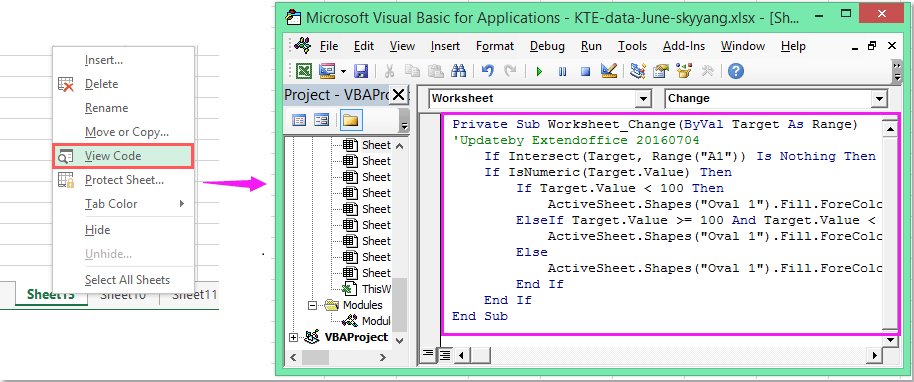
1. Haga clic derecho en la pestaña de la hoja en la que desea cambiar el color de la forma y luego seleccione Ver código en el menú contextual, en el emergente Microsoft Visual Basic para aplicaciones ventana, copie y pegue el siguiente código en el espacio en blanco Módulo ventana.

Código de VBA: cambie el color de la forma según el valor de la celda:

Private Sub Worksheet_Change(ByVal Target As Range)
'Updateby Extendoffice 20160704
    If Intersect(Target, Range("A1")) Is Nothing Then Exit Sub
    If IsNumeric(Target.Value) Then
        If Target.Value < 100 Then
            ActiveSheet.Shapes("Oval 1").Fill.ForeColor.RGB = vbRed
        ElseIf Target.Value >= 100 And Target.Value < 200 Then
            ActiveSheet.Shapes("Oval 1").Fill.ForeColor.RGB = vbYellow
        Else
            ActiveSheet.Shapes("Oval 1").Fill.ForeColor.RGB = vbGreen
        End If
    End If
End Sub

doc cambiar forma color 2

2. Y luego, cuando ingrese el valor en la celda A1, el color de la forma se cambiará con el valor de celda como lo definió.

Note: En el código anterior, A1 es el valor de celda en el que se cambiaría el color de su forma, y ​​el Oval 1 es el nombre de la forma de su forma insertada, puede cambiarlos según sus necesidades.

Las mejores herramientas de productividad de oficina

🤖 Asistente de IA de Kutools: Revolucionar el análisis de datos basado en: Ejecución inteligente   |  Generar codigo  |  Crear fórmulas personalizadas  |  Analizar datos y generar gráficos  |  Invocar funciones de Kutools...
Características populares: Buscar, resaltar o identificar duplicados   |  Eliminar filas en blanco   |  Combine columnas o celdas sin perder datos   |   Ronda sin fórmula ...
Super búsqueda: Búsqueda virtual de criterios múltiples    Búsqueda V de valores múltiples  |   VLookup en varias hojas   |   Búsqueda difusa ....
Lista desplegable avanzada: Crear rápidamente una lista desplegable   |  Lista desplegable dependiente   |  Lista desplegable de selección múltiple ....
Administrador de columnas: Agregar un número específico de columnas  |  Mover columnas  |  Toggle Estado de visibilidad de columnas ocultas  |  Comparar rangos y columnas ...
Características destacadas: Enfoque de cuadrícula   |  Vista de diseño   |   Gran barra de fórmulas    Administrador de hojas y libros de trabajo   |  Biblioteca de Recursos (Texto automático)   |  Selector de fechas   |  Combinar hojas de trabajo   |  Cifrar/descifrar celdas    Enviar correos electrónicos por lista   |  Súper filtro   |   Filtro especial (filtro negrita/cursiva/tachado...) ...
Los 15 mejores conjuntos de herramientas12 Texto Herramientas (Añadir texto, Quitar caracteres, ...)   |   50+ Tabla Tipos (Diagrama de Gantt, ...)   |   40+ Práctico Fórmulas (Calcular la edad según el cumpleaños, ...)   |   19 Inserción Herramientas (Insertar código QR, Insertar imagen desde la ruta, ...)   |   12 Conversión Herramientas (Números a palabras, Conversión de Moneda, ...)   |   7 Fusionar y dividir Herramientas (Filas combinadas avanzadas, Células partidas, ...)   |   ... y más

Mejore sus habilidades de Excel con Kutools for Excel y experimente la eficiencia como nunca antes. Kutools for Excel ofrece más de 300 funciones avanzadas para aumentar la productividad y ahorrar tiempo.  Haga clic aquí para obtener la función que más necesita...

Descripción


Office Tab lleva la interfaz con pestañas a Office y hace que su trabajo sea mucho más fácil

  • Habilite la edición y lectura con pestañas en Word, Excel, PowerPoint, Publisher, Access, Visio y Project.
  • Abra y cree varios documentos en nuevas pestañas de la misma ventana, en lugar de en nuevas ventanas.
  • ¡Aumenta su productividad en un 50% y reduce cientos de clics del mouse todos los días!
Comments (22)
Rated 4 out of 5 · 1 ratings
This comment was minimized by the moderator on the site
how would be the VBA code to paint several autoforms according to a range of data?
the values are in column B and I have 20 autoforms.
This comment was minimized by the moderator on the site
Como faço para para variar as cores da forma se minha opções for em formato de texto, como "Sim" e "Não"?
This comment was minimized by the moderator on the site
Hello, Emilly
To solve your problem, please apply the below code:
Private Sub Worksheet_Change(ByVal Target As Range)
If Range("A1") = "Yes" Then
ActiveSheet.Shapes("Oval 1").Fill.ForeColor.RGB = vbRed
Else
If Range("A1") = "No" Then
ActiveSheet.Shapes("Oval 1").Fill.ForeColor.RGB = vbGreen
End If
End If
End Sub


Please have a try, hope it can help you!
This comment was minimized by the moderator on the site
Hi Skyyang,

I tried the original VBA code and got it to work, although it would not activate actively when the cell changed. Today the code is not working and I also tried your more simplistic code and still did not work. The only thing that changed is that I copied the worksheet which contained the code that worked. Would this then result in it not working?
This comment was minimized by the moderator on the site
Hola, excelente ejemplo.
Pero como seria si tengo una forma y quiero ir coloreado poco a poco dependiendo del valor ejemplo:
Si el valor es 50%
Seia mitad roja y mitad verde
Pero que se vaya llenando según el porcentaje vaya aumentando
Rated 4 out of 5
This comment was minimized by the moderator on the site
I am new to VBAs and am struggling with something. I need to have 9 different cells A1-A9 change the colour of 9 different objects. Objects are cubes 1-9. Just to clarify, each cell is to change just one object A1-Cube 1, etc. Red if it fails to meet the value and green if it exceeds the value. The pass/fail value can change so instead of having the value in the VBA I need it to reference cell A10 which has the pass/fail value. Any chance someone could through out a sample code for me to work with.

Thanks
This comment was minimized by the moderator on the site
Great solution! How can I do if I have more than 1 oval in the worksheet which the colors change according to the value input say in A1, B1,C1? Thanks in advance for your reply! 
This comment was minimized by the moderator on the site
Hello mnsosa,Glad to help. Please copy and paste the below VBA code into the blank Module window.
Sub TestMacro2()
Dim dblHt As Double
Dim rngC As Range
Dim lngr As Long
Dim dblMargin As Double
Dim lngSR As Long

lngSR = 2 'Row where the data starts

dblMargin = 6 ' Distance between shapes

'On Error Resume Next
ActiveSheet.Shapes.SelectAll
Selection.Delete
On Error GoTo 0


dblHt = Rows(lngSR).Height * 4

For lngr = lngSR To Cells(lngSR, "A").End(xlDown).Row
ActiveSheet.Shapes.AddShape(msoShapeOval, _
Cells(lngSR, "D").Left + ((lngr - lngSR) Mod 4) * dblHt + dblMargin, _
Cells(lngSR, "D").Top + Int((lngr - lngSR) / 4) * dblHt + dblMargin, _
dblHt - 2 * dblMargin, _
dblHt - 2 * dblMargin).Select
Selection.Name = "Round" & Cells(lngr, "A").Address
Selection.ShapeRange.TextFrame2.VerticalAnchor = msoAnchorMiddle
Selection.ShapeRange(1).TextFrame2.TextRange.Characters.Text = Cells(lngr, "A").Value
With Selection.ShapeRange(1).TextFrame2.TextRange.Characters(1, 2).ParagraphFormat
.FirstLineIndent = 0
.Alignment = msoAlignCenter
End With
With Selection.ShapeRange(1).TextFrame2.TextRange.Characters(1, 2).Font
.Bold = msoTrue
.Fill.Visible = msoTrue
.Fill.ForeColor.ObjectThemeColor = msoThemeColorText1
.Fill.ForeColor.TintAndShade = 0
.Fill.ForeColor.Brightness = 0
.Fill.Transparency = 0
.Fill.Solid
.Size = 12
End With
With Selection.ShapeRange.Fill
.Visible = msoTrue
If Cells(lngr, "A").Value > 70 Then
.ForeColor.RGB = RGB(0, 176, 80)
ElseIf Cells(lngr, "A").Value >= 40 Then
.ForeColor.RGB = RGB(255, 255, 70)
Else
.ForeColor.RGB = RGB(255, 0, 0)
End If
.Transparency = 0
.Solid
End With
Next lngr
Range("A1").Select
End Sub

After you run the VBA code above, you will see multiple shapes are generated, and the colors of these shapes are changed according to the VBA.Please see my screenshot. Hope it can help. Have a nice day.Sincerely,Mandy
This comment was minimized by the moderator on the site
¿Cómo hacemos si tenemos más de 1 Oval en la hoja de trabajo cuyos colores cambian de acuerdo con el valor ingresado, por ejemplo, en A1, B1, C1...? Mil gracias por su ayuda!

This comment was minimized by the moderator on the site
Hello María Noel,
Glad to help. Please copy and paste the below VBA code into the blank Module window.

Sub TestMacro2()
Dim dblHt As Double
Dim rngC As Range
Dim lngr As Long
Dim dblMargin As Double
Dim lngSR As Long

lngSR = 2 'Row where the data starts

dblMargin = 6 ' Distance between shapes

'On Error Resume Next
ActiveSheet.Shapes.SelectAll
Selection.Delete
On Error GoTo 0


dblHt = Rows(lngSR).Height * 4

For lngr = lngSR To Cells(lngSR, "A").End(xlDown).Row
ActiveSheet.Shapes.AddShape(msoShapeOval, _
Cells(lngSR, "D").Left + ((lngr - lngSR) Mod 4) * dblHt + dblMargin, _
Cells(lngSR, "D").Top + Int((lngr - lngSR) / 4) * dblHt + dblMargin, _
dblHt - 2 * dblMargin, _
dblHt - 2 * dblMargin).Select
Selection.Name = "Round" & Cells(lngr, "A").Address
Selection.ShapeRange.TextFrame2.VerticalAnchor = msoAnchorMiddle
Selection.ShapeRange(1).TextFrame2.TextRange.Characters.Text = Cells(lngr, "A").Value
With Selection.ShapeRange(1).TextFrame2.TextRange.Characters(1, 2).ParagraphFormat
.FirstLineIndent = 0
.Alignment = msoAlignCenter
End With
With Selection.ShapeRange(1).TextFrame2.TextRange.Characters(1, 2).Font
.Bold = msoTrue
.Fill.Visible = msoTrue
.Fill.ForeColor.ObjectThemeColor = msoThemeColorText1
.Fill.ForeColor.TintAndShade = 0
.Fill.ForeColor.Brightness = 0
.Fill.Transparency = 0
.Fill.Solid
.Size = 12
End With
With Selection.ShapeRange.Fill
.Visible = msoTrue
If Cells(lngr, "A").Value > 70 Then
.ForeColor.RGB = RGB(0, 176, 80)
ElseIf Cells(lngr, "A").Value >= 40 Then
.ForeColor.RGB = RGB(255, 255, 70)
Else
.ForeColor.RGB = RGB(255, 0, 0)
End If
.Transparency = 0
.Solid
End With
Next lngr
Range("A1").Select
End Sub

After you run the VBA code above, you will see multiple shapes are generated, and the colors of these shapes are changed according to the VBA.
Please see my screenshot. Hope it can help. Have a nice day.
Sincerely,
Mandy
This comment was minimized by the moderator on the site
Hi... excellent solution... but how do I apply it to multiple shapes based on the corresponding values of a range of cells. Many thanks in advance for your help.
This comment was minimized by the moderator on the site
Hello Ryan,
Glad to help. Please copy and paste the below VBA code into the blank Module window.

Sub TestMacro2()
Dim dblHt As Double
Dim rngC As Range
Dim lngr As Long
Dim dblMargin As Double
Dim lngSR As Long

lngSR = 2 'Row where the data starts

dblMargin = 6 ' Distance between shapes

'On Error Resume Next
ActiveSheet.Shapes.SelectAll
Selection.Delete
On Error GoTo 0


dblHt = Rows(lngSR).Height * 4

For lngr = lngSR To Cells(lngSR, "A").End(xlDown).Row
ActiveSheet.Shapes.AddShape(msoShapeOval, _
Cells(lngSR, "D").Left + ((lngr - lngSR) Mod 4) * dblHt + dblMargin, _
Cells(lngSR, "D").Top + Int((lngr - lngSR) / 4) * dblHt + dblMargin, _
dblHt - 2 * dblMargin, _
dblHt - 2 * dblMargin).Select
Selection.Name = "Round" & Cells(lngr, "A").Address
Selection.ShapeRange.TextFrame2.VerticalAnchor = msoAnchorMiddle
Selection.ShapeRange(1).TextFrame2.TextRange.Characters.Text = Cells(lngr, "A").Value
With Selection.ShapeRange(1).TextFrame2.TextRange.Characters(1, 2).ParagraphFormat
.FirstLineIndent = 0
.Alignment = msoAlignCenter
End With
With Selection.ShapeRange(1).TextFrame2.TextRange.Characters(1, 2).Font
.Bold = msoTrue
.Fill.Visible = msoTrue
.Fill.ForeColor.ObjectThemeColor = msoThemeColorText1
.Fill.ForeColor.TintAndShade = 0
.Fill.ForeColor.Brightness = 0
.Fill.Transparency = 0
.Fill.Solid
.Size = 12
End With
With Selection.ShapeRange.Fill
.Visible = msoTrue
If Cells(lngr, "A").Value > 70 Then
.ForeColor.RGB = RGB(0, 176, 80)
ElseIf Cells(lngr, "A").Value >= 40 Then
.ForeColor.RGB = RGB(255, 255, 70)
Else
.ForeColor.RGB = RGB(255, 0, 0)
End If
.Transparency = 0
.Solid
End With
Next lngr
Range("A1").Select
End Sub

After you run the VBA code above, you will see multiple shapes are generated, and the colors of these shapes are changed according to the VBA.
Please see my screenshot. Hope it can help. Have a nice day.
Sincerely,
Mandy
This comment was minimized by the moderator on the site
How do I make the private sub to read the result from the AVERAGE(C1,C5,C9) calculation?

Sub only works with numeric values; any thoughts and suggestions are greatly appreciated.
This comment was minimized by the moderator on the site
Hello Cesare,How are you? I notice that the VBA code can work with the AVERAGE(number, number...) calculation. But the trick is that every time you change the values in the calculation, you need to double-click the formula in the cell to make the VBA work again. 
For example, In cell A1, after we input the formula is =AVERAGE(C2:D3), the VBA works and changes the color of the shape accordingly. Please see screenshot 1. <span style="letter-spacing: 0.2px; color: inherit; font-family: inherit; font-style: inherit; font-variant-ligatures: inherit; font-variant-caps: inherit; font-weight: inherit;">C2:D3, the returned result in cell A1 changes, but the shape color hasn't been changed yet. In this case, we need to double click the formula in cell A1 to make the VBA work. Then the shape color will be changed accordingly. Please see screenshots 2 and 3.</span>
This comment was minimized by the moderator on the site
Thanks for this which is really useful.

I now want to use it with a pivot table on another worksheet which controls the data on the sheet with the shapes that I want to change colour. However, when I change the selection on the pivot table the data on the worksheet with the shapes is updated but the code does not run so the shapes do not change colour

If I manually change the values the code runs and the colour of the shapes is updated.

Question: what do i need to add to the code above to allow it to run automatically?
This comment was minimized by the moderator on the site
How can this be applied if you have multiple shape in the same worksheet?
This comment was minimized by the moderator on the site
Hello Yasir,
Glad to help. Please copy and paste the below VBA code into the blank Module window.

Sub TestMacro2()
Dim dblHt As Double
Dim rngC As Range
Dim lngr As Long
Dim dblMargin As Double
Dim lngSR As Long

lngSR = 2 'Row where the data starts

dblMargin = 6 ' Distance between shapes

'On Error Resume Next
ActiveSheet.Shapes.SelectAll
Selection.Delete
On Error GoTo 0


dblHt = Rows(lngSR).Height * 4

For lngr = lngSR To Cells(lngSR, "A").End(xlDown).Row
ActiveSheet.Shapes.AddShape(msoShapeOval, _
Cells(lngSR, "D").Left + ((lngr - lngSR) Mod 4) * dblHt + dblMargin, _
Cells(lngSR, "D").Top + Int((lngr - lngSR) / 4) * dblHt + dblMargin, _
dblHt - 2 * dblMargin, _
dblHt - 2 * dblMargin).Select
Selection.Name = "Round" & Cells(lngr, "A").Address
Selection.ShapeRange.TextFrame2.VerticalAnchor = msoAnchorMiddle
Selection.ShapeRange(1).TextFrame2.TextRange.Characters.Text = Cells(lngr, "A").Value
With Selection.ShapeRange(1).TextFrame2.TextRange.Characters(1, 2).ParagraphFormat
.FirstLineIndent = 0
.Alignment = msoAlignCenter
End With
With Selection.ShapeRange(1).TextFrame2.TextRange.Characters(1, 2).Font
.Bold = msoTrue
.Fill.Visible = msoTrue
.Fill.ForeColor.ObjectThemeColor = msoThemeColorText1
.Fill.ForeColor.TintAndShade = 0
.Fill.ForeColor.Brightness = 0
.Fill.Transparency = 0
.Fill.Solid
.Size = 12
End With
With Selection.ShapeRange.Fill
.Visible = msoTrue
If Cells(lngr, "A").Value > 70 Then
.ForeColor.RGB = RGB(0, 176, 80)
ElseIf Cells(lngr, "A").Value >= 40 Then
.ForeColor.RGB = RGB(255, 255, 70)
Else
.ForeColor.RGB = RGB(255, 0, 0)
End If
.Transparency = 0
.Solid
End With
Next lngr
Range("A1").Select
End Sub

After you run the VBA code above, you will see multiple shapes are generated, and the colors of these shapes are changed according to the VBA.
Please see my screenshot. Hope it can help. Have a nice day.
Sincerely,
Mandy
There are no comments posted here yet
Load More
Please leave your comments in English
Posting as Guest
×
Rate this post:
0   Characters
Suggested Locations