¿Cómo encontrar la enésima celda no vacía en Excel?
¿Cómo puede encontrar y devolver el valor de la enésima celda no vacía de una columna o fila en Excel? En este artículo, le presentamos fórmulas prácticas que le ayudarán a lograrlo con facilidad.
Encontrar y devolver el valor de la enésima celda no vacía de una columna con una fórmula
Encontrar y devolver el valor de la enésima celda no vacía de una fila con una fórmula
 Encontrar y devolver el valor de la enésima celda no vacía de una columna con una fórmula
Por ejemplo, tengo una columna de datos como la que se muestra en la siguiente captura de pantalla; ahora obtendré el valor de la tercera celda no vacía de esta lista.
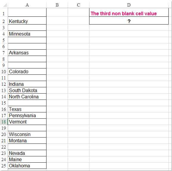
Introduzca esta fórmula:=INDEX($A$1:$A$25,SMALL(ROW($A$1:$A$25)+(100*($A$1:$A$25=«»)), 3))&""en una celda vacía donde desee mostrar el resultado, por ejemplo, D2, y después pulse las teclas Ctrl + Mayús + Entrarsimultáneamente para obtener el resultado correcto; consulte la captura de pantalla:

Nota: En la fórmula anterior, A1:A25 es el rango de datos que desea utilizar, y el número 3 indica el valor de la tercera celda no vacía que se devolverá. Si desea obtener la segunda celda no vacía, basta con cambiar el número 3 por 2 según sus necesidades.
Encontrar y devolver el valor de la enésima celda no vacía de una fila con una fórmula
Si desea encontrar y devolver el valor de la enésima celda no vacía en una fila, la siguiente fórmula puede ayudarle; proceda de la siguiente manera:
Introduzca esta fórmula:=INDEX($A$1:$M$1,SMALL(IF($A$1:$M$1<>«»,COLUMN($A$1:$M$1)-COLUMN($A$1)+1),4))en una celda vacía donde desee colocar el resultado y, a continuación, pulse las teclas Ctrl + Mayús + Entrarsimultáneamente para obtener el resultado; consulte la captura de pantalla:
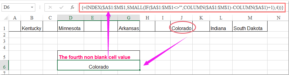
Nota: En la fórmula anterior, A1:M1 son los valores de la fila que desea utilizar, y el número 4 indica el valor de la cuarta celda no vacía que desea devolver. Si quiere obtener la segunda celda no vacía, basta con cambiar el número 4 por 2 según necesite.
Las mejores herramientas de productividad para Office
Potencie sus habilidades en Excel con Kutools para Excel y experimente una eficiencia como nunca antes.Kutools para Excel ofrece más de 300 funciones avanzadas para aumentar su productividad y Ahorrar tiempo.Haga clic aquí para obtener la función que más necesita...
Office Tab aporta una interfaz con pestañas a Office y hace que su trabajo sea mucho más fácil
- Active la edición y lectura con pestañas en Word, Excel, PowerPoint, Publisher, Access, Visio y Project.
- Abra y cree varios documentos en nuevas pestañas dentro de la misma ventana, en lugar de hacerlo en ventanas separadas.
- ¡Aumente su productividad en un 50 % y elimine cientos de clics del ratón cada día!
Todos los complementos de Kutools en un solo instalador.
Kutools for Office es la suite que incluye complementos para Excel, Word, Outlook y PowerPoint, además de Office Tab Pro, ideal para equipos que trabajan en distintas aplicaciones de Office.
- Suite integral— complementos para Excel, Word, Outlook y PowerPoint + Office Tab Pro
- Un instalador, una licencia— configuración en minutos (compatible con MSI)
- Rendimiento mejorado en conjunto— productividad optimizada en todas las aplicaciones de Office
- Prueba gratuita de 30 días con todas las funciones— sin registro ni tarjeta de crédito
- La mejor relación calidad-precio— ahorre frente a la compra individual de complementos