¿Cómo resaltar una celda o una fila mediante una casilla de verificación en Excel?
Como se muestra en la siguiente captura de pantalla, debe resaltar una fila o una celda mediante una casilla de verificación. Al marcarla, la fila o celda indicada se resaltará automáticamente. ¿Pero cómo lograrlo en Excel? Este artículo le presenta dos métodos para conseguirlo.

Resaltar celda o fila con casilla de verificación mediante Usar formato condicional
Resaltar celda o fila con casilla de verificación mediante código VBA
Resaltar celda o fila con casilla de verificación mediante Usar formato condicional
Puede crear una regla de formato condicional para resaltar una celda o una fila mediante una casilla de verificación en Excel. Siga estos pasos.
PASO UNO: Vincule todas las Casilla de Verificación a una celda específica
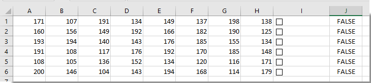
1. Debe insertar casillas de verificación en las celdas una por una manualmente haciendo clic en Programador > Insertar > Casilla de verificación (Control de formulario).
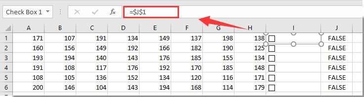
2. Ahora se han insertado casillas de verificación en las celdas de la columna I. Haz clic en la primera casilla de verificación en I1, introduce la fórmula =$J1 en la barra de fórmulas y, a continuación, pulsa la tecla Entrar.
Consejo: Si no quiere que aparezcan valores asociados en las celdas adyacentes a las casillas de verificación, puede vincular la casilla a una celda de otra hoja de cálculo, por ejemplo, =Hoja3!$E1.
3. Repita el paso 1 hasta que todas las casillas de verificación estén vinculadas a celdas adyacentes o a celdas de otra hoja de cálculo.
Nota: Todas las celdas vinculadas deben ser consecutivas y estar situadas en la misma columna.
PASO DOS: Cree una regla de Usar formato condicional
Ahora debe crear una regla de formato condicional siguiendo los pasos que se indican a continuación.
1. Seleccione las filas que desea resaltar con casillas de verificación y, a continuación, haga clic en Usar formato condicional > Nueva regla en la pestaña Inicio. Vea la captura de pantalla:

2. En el cuadro de diálogo Nueva regla de formato, debe:
2,1 Seleccione la opción Usar una fórmula para determinar qué celdas aplicar formatoen el cuadro Seleccionar un tipo de regla;
2,2 Introduzca la fórmula =SI($J1=VERDADERO;VERDADERO;FALSO) en el cuadro Aplicar formato a los valores donde esta fórmula sea verdadera;
o bien =SI(Hoja3!$E1=VERDADERO;VERDADERO;FALSO) si la casilla de verificación está vinculada a otra hoja de cálculo.
2,3 Haga clic en el botón Formatopara especificar un color de resaltado para las filas;
2,4 Haga clic en el botón Aceptar. Vea la captura de pantalla:

Nota: En la fórmula, $J1 o $E1es la primera celda vinculada a la casilla de verificación. Asegúrese de que la referencia de celda se haya cambiado a absoluta en la columna ()J1 > $J1 o E1 > $E1).
Ahora se ha creado la regla de formato condicional. Al marcar las casillas de verificación, las filas correspondientes se resaltarán automáticamente, tal como se muestra en la siguiente captura de pantalla.

Resaltar celda o fila con casilla de verificación mediante código VBA
El siguiente código VBA también le permite resaltar una celda o una fila mediante una casilla de verificación en Excel. Siga estos pasos.
1. En la hoja de cálculo en la que desea resaltar una celda o una fila con una casilla de verificación, haga clic con el botón derecho en la pestaña de hoja y seleccione Ver código en el menú contextual para abrir la ventana de Microsoft Visual Basic para Aplicaciones.
2. A continuación, copie y pegue el siguiente código VBA en la ventana de código.
Código VBA: Resaltar fila con casilla de verificación en Excel
Sub AddCheckBox()
Dim xCell As Range
Dim xRng As Range
Dim I As Integer
Dim xChk As CheckBox
On Error Resume Next
InputC:
    Set xRng = Application.InputBox("Please select the column range to insert checkboxes:", "Kutools for Excel", Selection.Address, , , , , 8)
If xRng Is Nothing Then Exit Sub
If xRng.Columns.Count > 1 Then
    MsgBox "The selected range should be a single column", vbInformation, "Kutools fro Excel"
    GoTo InputC
Else
    If xRng.Columns.Count = 1 Then
        For Each xCell In xRng
            With ActiveSheet.CheckBoxes.Add(xCell.Left, _
               xCell.Top, xCell.Width = 15, xCell.Height = 12)
               .LinkedCell = xCell.Offset(, 1).Address(External:=False)
               .Interior.ColorIndex = xlNone
               .Caption = ""
               .Name = "Check Box " & xCell.Row
            End With
            xRng.Rows(xCell.Row).Interior.ColorIndex = xlNone
        Next
    End If
    With xRng
     .Rows.RowHeight = 16
    End With
    xRng.ColumnWidth = 5#
    xRng.Cells(1, 1).Offset(0, 1).Select
    For Each xChk In ActiveSheet.CheckBoxes
      xChk.OnAction = ActiveSheet.Name + ".InsertBgColor"
    Next
End If
End Sub

Sub InsertBgColor()
Dim xName As Integer
Dim xChk As CheckBox
For Each xChk In ActiveSheet.CheckBoxes
  xName = Right(xChk.Name, Len(xChk.Name) - 10)
  If (xName = Range(xChk.LinkedCell).Row) Then
   If (Range(xChk.LinkedCell) = "True") Then
    Range("A" & xName, Range(xChk.LinkedCell).Offset(0, -2)).Interior.ColorIndex = 6
   Else
    Range("A" & xName, Range(xChk.LinkedCell).Offset(0, -2)).Interior.ColorIndex = xlNone
   End If
  End If
Next
End Sub
3. Pulse la tecla F5para ejecutar el código. ()Nota: debe colocar el cursor en la primera parte del código para poder usar la tecla F5). En el cuadro de diálogo Kutools para Excel que aparece, seleccione el rango en el que desea insertar casillas de verificación y, a continuación, haga clic en el botón Aceptar. En este caso, se ha seleccionado I1:I6. Vea la captura de pantalla:

4. A continuación, se insertan casillas de verificación en las celdas seleccionadas. Al marcar cualquiera de ellas, la fila correspondiente se resaltará automáticamente, tal como se muestra en la siguiente captura de pantalla.

Artículos relacionados:
- ¿Cómo cambiar el valor o el color de una celda específica al marcar una casilla de verificación en Excel?
- ¿Cómo insertar la fecha en una celda al marcar una casilla de verificación en Excel?
- ¿Cómo marcar automáticamente una casilla de verificación en Excel según el valor de una celda?
- ¿Cómo filtrar datos según el estado de una casilla de verificación en Excel?
- ¿Cómo ocultar una casilla de verificación al ocultar su fila en Excel?
- ¿Cómo crear una lista desplegable con varias casillas de verificación en Excel?
Las mejores herramientas de productividad para Office
Potencie sus habilidades en Excel con Kutools para Excel y experimente una eficiencia como nunca antes.Kutools para Excel ofrece más de 300 funciones avanzadas para aumentar su productividad y Ahorrar tiempo.Haga clic aquí para obtener la función que más necesita...
Office Tab aporta una interfaz con pestañas a Office y hace que su trabajo sea mucho más fácil
- Active la edición y lectura con pestañas en Word, Excel, PowerPoint, Publisher, Access, Visio y Project.
- Abra y cree varios documentos en nuevas pestañas dentro de la misma ventana, en lugar de hacerlo en ventanas separadas.
- ¡Aumente su productividad en un 50 % y elimine cientos de clics del ratón cada día!
Todos los complementos de Kutools en un solo instalador.
Kutools for Office es la suite que incluye complementos para Excel, Word, Outlook y PowerPoint, además de Office Tab Pro, ideal para equipos que trabajan en distintas aplicaciones de Office.
- Suite integral— complementos para Excel, Word, Outlook y PowerPoint + Office Tab Pro
- Un instalador, una licencia— configuración en minutos (compatible con MSI)
- Rendimiento mejorado en conjunto— productividad optimizada en todas las aplicaciones de Office
- Prueba gratuita de 30 días con todas las funciones— sin registro ni tarjeta de crédito
- La mejor relación calidad-precio— ahorre frente a la compra individual de complementos