¿Cómo sumar valores en Excel según criterios de fila y columna?
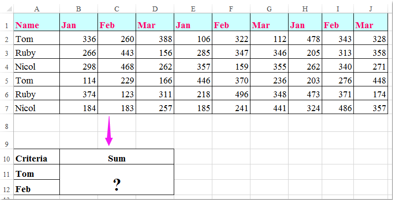
Tengo un rango de datos que contiene encabezados de fila y de columna, y ahora quiero obtener la suma de las celdas que cumplen simultáneamente los criterios de encabezado de columna y de fila. Por ejemplo, sumar las celdas cuyo criterio de columna es Tom y el criterio de fila es febrero, tal como se muestra en la siguiente captura de pantalla. En este artículo, explicaré algunas fórmulas útiles para resolverlo.
Sumar celdas según criterios de columna y fila con fórmulas
 Sumar celdas según criterios de columna y fila con fórmulas
Aquí puede aplicar las siguientes fórmulas para sumar celdas según ambos criterios (columna y fila). Siga estos pasos:
Introduzca cualquiera de las fórmulas siguientes en una celda vacía donde desee mostrar el resultado:
=SUMPRODUCT((A2:A7="Tom")*(B1:J1="Feb")*(B2:J7))
=SUM(IF(B1:J1="Feb",IF(A2:A7="Tom",B2:J7)))
Y luego pulse Mayús + Ctrl + Introsimultáneamente para obtener el resultado, consulte la captura de pantalla:
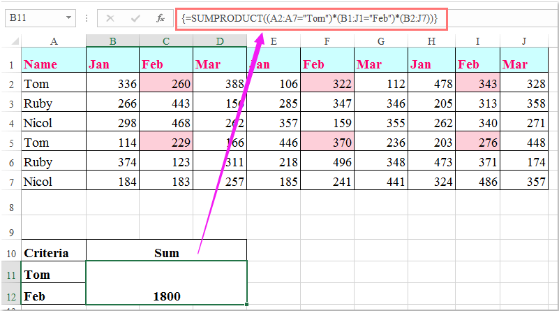
Nota: En las fórmulas anteriores, Tom y feb son los criterios de columna y fila sobre los que se basa la suma; A2:A7 y B1:J1 son los encabezados de columna y de fila que contienen dichos criterios, y B2:J7 es el rango de datos que desea sumar.

Descubra la magia de Excel con KUTOOLS AI
- Ejecución inteligente: Realice operaciones en celdas, analice datos y cree gráficos con comandos sencillos.
- fórmulas personalizadas: Cree fórmulas a medida para optimizar sus flujos de trabajo.
- Programación en VBA: Escriba e implemente código VBA con facilidad.
- Interpretación de fórmulas: Entienda las fórmulas complejas con facilidad.
- Traducción de texto: Rompa las barreras del idioma directamente en sus hojas de cálculo.
Las mejores herramientas de productividad para Office
Potencie sus habilidades en Excel con Kutools para Excel y experimente una eficiencia como nunca antes.Kutools para Excel ofrece más de 300 funciones avanzadas para aumentar su productividad y Ahorrar tiempo.Haga clic aquí para obtener la función que más necesita...
Office Tab aporta una interfaz con pestañas a Office y hace que su trabajo sea mucho más fácil
- Active la edición y lectura con pestañas en Word, Excel, PowerPoint, Publisher, Access, Visio y Project.
- Abra y cree varios documentos en nuevas pestañas dentro de la misma ventana, en lugar de hacerlo en ventanas separadas.
- ¡Aumente su productividad en un 50 % y elimine cientos de clics del ratón cada día!
Todos los complementos de Kutools en un solo instalador.
Kutools for Office es la suite que incluye complementos para Excel, Word, Outlook y PowerPoint, además de Office Tab Pro, ideal para equipos que trabajan en distintas aplicaciones de Office.
- Suite integral— complementos para Excel, Word, Outlook y PowerPoint + Office Tab Pro
- Un instalador, una licencia— configuración en minutos (compatible con MSI)
- Rendimiento mejorado en conjunto— productividad optimizada en todas las aplicaciones de Office
- Prueba gratuita de 30 días con todas las funciones— sin registro ni tarjeta de crédito
- La mejor relación calidad-precio— ahorre frente a la compra individual de complementos