¿Cómo crear una lista desplegable dependiente en Google Sheets?
Insertar una lista desplegable estándar en Google Sheets puede parecer sencillo, pero a veces necesitarás crear una lista dinámica, en la que las opciones de la segunda dependan de la selección realizada en la primera. ¿Cómo podrías lograrlo en Google Sheets?
Crear una lista desplegable dependiente en Google Sheets
Crear una lista desplegable dependiente en Google Sheets
Siga estos pasos para crear una Lista dinámica en Google Sheets:
1. En primer lugar, inserte la lista desplegable básica: seleccione una celda donde quiera colocar la primera lista desplegable y, a continuación, haga clic en Datos > Validación de datos. Consulte la captura de pantalla:

2. En el cuadro de diálogo emergente Validación de datos, seleccione Lista de un intervalo en la lista desplegable situada junto a la sección Criterios y, a continuación, haga clic en el botón para seleccionar los valores de celda sobre los que desea crear la primera lista desplegable. Consulte la captura de pantalla: 

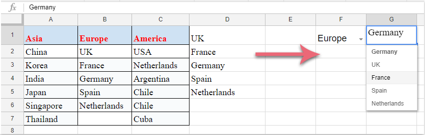
3. A continuación, haga clic en el botón Guardar; así se habrá creado la primera lista desplegable. Seleccione un elemento de la lista desplegable creada e introduzca esta fórmula: =arrayformula(if(F1=A1,A2:A7,if(F1=B1,B2:B6,if(F1=C1,C2:C7,«»)))) en una celda vacía adyacente a las columnas de datos y pulse la tecla Intro. De este modo, se mostrarán inmediatamente todos los valores coincidentes según el elemento seleccionado en la primera lista desplegable. Consulte la captura de pantalla:
Nota: En la fórmula anterior, F1 es la celda de la primera lista desplegable; A1, B1 y C1 son los elementos de la primera lista desplegable; y A2:A7, B2:B6 y C2:C7 son los rangos de celdas en los que se basa la segunda lista desplegable. Puede ajustarlos según sus necesidades.

4. A continuación, cree la segunda lista desplegable dependiente: haga clic en la celda donde quiera colocarla y, después, vaya a Datos > Validación de datos para abrir el cuadro de diálogo Validación de datos. En la sección Criterios, seleccione Lista de un intervalo en el menú desplegable y, a continuación, haga clic en el botón para elegir las celdas que contienen la fórmula con los resultados coincidentes del elemento seleccionado en la primera lista desplegable. Consulte la captura de pantalla:

5. Por último, haga clic en el botón Guardar y la segunda lista desplegable dependiente quedará creada correctamente, tal como se muestra en la siguiente captura de pantalla:
Las mejores herramientas de productividad para Office
Potencie sus habilidades en Excel con Kutools para Excel y experimente una eficiencia como nunca antes.Kutools para Excel ofrece más de 300 funciones avanzadas para aumentar su productividad y Ahorrar tiempo.Haga clic aquí para obtener la función que más necesita...
Office Tab aporta una interfaz con pestañas a Office y hace que su trabajo sea mucho más fácil
- Active la edición y lectura con pestañas en Word, Excel, PowerPoint, Publisher, Access, Visio y Project.
- Abra y cree varios documentos en nuevas pestañas dentro de la misma ventana, en lugar de hacerlo en ventanas separadas.
- ¡Aumente su productividad en un 50 % y elimine cientos de clics del ratón cada día!
Todos los complementos de Kutools en un solo instalador.
Kutools for Office es la suite que incluye complementos para Excel, Word, Outlook y PowerPoint, además de Office Tab Pro, ideal para equipos que trabajan en distintas aplicaciones de Office.
- Suite integral— complementos para Excel, Word, Outlook y PowerPoint + Office Tab Pro
- Un instalador, una licencia— configuración en minutos (compatible con MSI)
- Rendimiento mejorado en conjunto— productividad optimizada en todas las aplicaciones de Office
- Prueba gratuita de 30 días con todas las funciones— sin registro ni tarjeta de crédito
- La mejor relación calidad-precio— ahorre frente a la compra individual de complementos