¿Cómo usar el formato condicional en Google Sheets basado en valores de otra hoja?
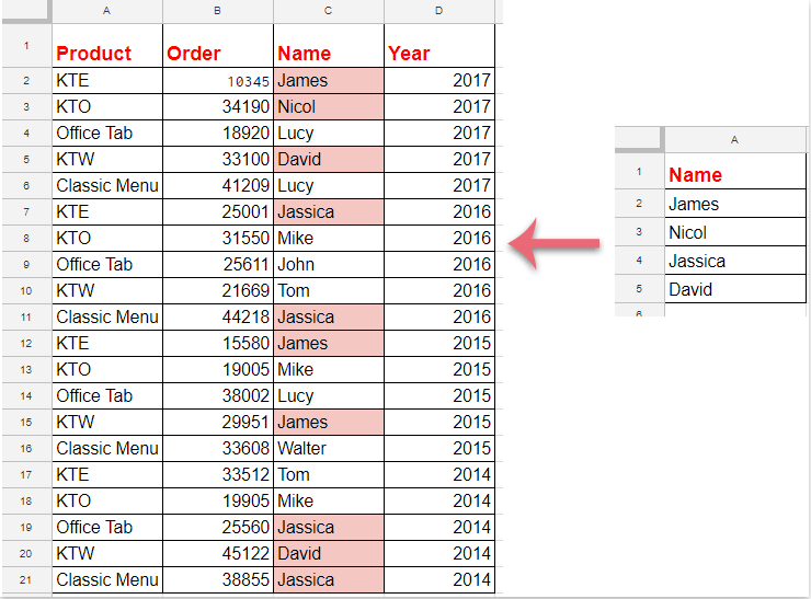
El formato condicional es una función útil en Google Sheets que le permite resaltar automáticamente celdas según criterios específicos, facilitando así el análisis y la visualización de sus datos. A veces, en lugar de basar el resaltado en valores de la misma hoja, puede necesitar crear reglas que hagan referencia a una lista o criterios almacenados en otra hoja. Por ejemplo, podría querer resaltar celdas en una hoja si coinciden con elementos de una lista mantenida en otra hoja, tal como se muestra en la siguiente captura de pantalla. Este tipo de tarea es habitual al trabajar con datos cruzados, como comparar ventas actuales con una lista maestra de productos o identificar entradas duplicadas frente a otro rango de origen. Sin embargo, configurar este tipo de formato condicional en Google Sheets —especialmente al hacer referencia a datos entre hojas— puede resultar confuso si no lo ha hecho antes. La guía siguiente le mostrará, paso a paso, un enfoque sencillo para lograrlo.
Guía para resaltar celdas basándose en una lista de otra hoja en Google Sheets
Tutorial para resaltar celdas basándose en una lista de otra hoja en Google Sheets
Este método le permite configurar una regla de formato condicional para resaltar celdas en su hoja de cálculo actual si aparecen en una lista especificada en otra hoja. Este tipo de formato condicional entre hojas resulta especialmente útil para el seguimiento dinámico de datos y para mantener la coherencia entre conjuntos de datos relacionados.
Para completar este proceso, siga estos pasos detallados:
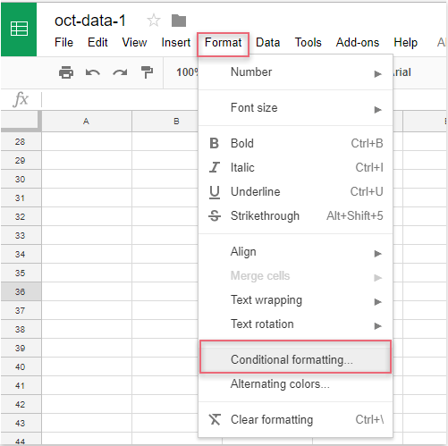
1. Abra su hoja de trabajo de destino, haga clic en el menú Formato situado en la parte superior y seleccione Usar formato condicional. Se abrirá el panel de reglas de Formato condicional en el lado derecho de su pantalla.
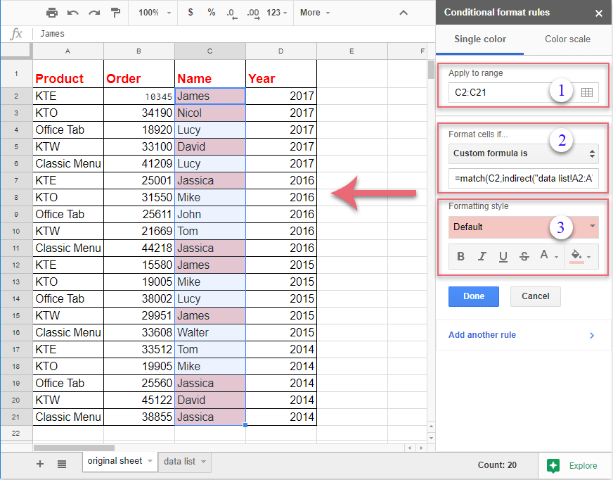
2. En el panel de Formato condicional, realice las siguientes acciones:
(1.) Haga clic en el botón  situado junto al campo «Aplicar al rango». Seleccione el rango de celdas que desea resaltar. Por ejemplo, si quiere aplicar formato a todos los valores de la columna C desde la fila 2 hacia abajo, seleccione C2:C. Elegir un rango adecuado garantiza que solo se evalúen las celdas deseadas para aplicarles el formato.
(2.) En el menú desplegable Establecer formato de celda si, elija Fórmula personalizada es. Introduzca la siguiente fórmula en el cuadro proporcionado: =COINCIDIR(C2;INDIRECTO(«lista de datos!A2:A»);0). Esta fórmula comprueba si cada celda de la columna C coincide con algún valor del rango A2:A de la hoja «lista de datos».
(3.) En Estilo de formato, seleccione el formato deseado, como rellenar la celda con un color específico o cambiar el estilo de fuente. Podrá previsualizar el estilo directamente en su hoja antes de aplicarlo.
Nota: En la fórmula anterior, C2 hace referencia a la primera celda de su rango seleccionado (ajústela si sus datos comienzan en una fila o columna distinta), y lista de datos!A2:A hace referencia al nombre de la hoja (“lista de datos”) y al rango correspondiente (A2:A) donde se almacena su lista en otra hoja. Asegúrese de que la referencia de celda en la fórmula coincida con la primera celda situada a la izquierda de su rango seleccionado; de lo contrario, el formato podría no aplicarse correctamente. Si el rango de su lista de datos es distinto, recuerde actualizarlo en la fórmula (por ejemplo, “lista de datos!B2:B”).
3. Una vez configurada la regla, las celdas coincidentes en el rango seleccionado se resaltarán al instante según la lista de la otra hoja. Revise la vista previa y, a continuación, haga clic en Listo en la parte inferior del panel de reglas de Formato condicional para aplicar y guardar su formato.
Consejos y solución de problemas:
- Compruebe cuidadosamente si hay errores tipográficos en su fórmula, especialmente en los nombres de hojas y las referencias de rango; las referencias incorrectas son una causa habitual por la que las reglas no se aplican.
- Si su lista de datos contiene celdas vacías, la función
COINCIDIRdevolverá un error#N/Apara los valores que no coincidan, pero este comportamiento es el esperado y no afecta al resaltado de los elementos coincidentes. - Cuando copie el formato a una hoja nueva o ajuste los rangos, asegúrese de actualizar también las referencias de celda en su fórmula personalizada en consecuencia.
- El formato se actualiza automáticamente si posteriormente añade o elimina elementos de su lista de referencia.
- La hoja y el rango a los que hace referencia su fórmula existen y están escritos correctamente.
- La primera celda de su fórmula coincide con la primera celda del rango seleccionado.
- Dispone de todos los permisos necesarios para acceder entre hojas dentro de su hoja de cálculo; este método solo funciona dentro de un único archivo de Google Sheets que contenga varias hojas, no entre archivos distintos.
Como alternativa, si su estructura de datos o requisitos son más complejos —por ejemplo, si necesita comparar varias columnas, permitir coincidencias parciales o realizar búsquedas más avanzadas—, puede emplear columnas auxiliares con fórmulas CONTAR.SI o BUSCARV, o utilizar Google Apps Script (código JavaScript personalizado) para lograr soluciones flexibles con formato condicional.
En resumen, configurar el formato condicional basado en otra hoja resulta altamente eficaz para comprobaciones de listas, seguimiento de duplicados y diversas validaciones de datos entre hojas, todo ello directamente en Google Sheets. Asegúrese siempre de verificar las entradas de su fórmula, los rangos de referencia y las reglas de formato para obtener resultados fluidos y precisos.

Descubra la magia de Excel con KUTOOLS AI
- Ejecución inteligente: Realice operaciones en celdas, analice datos y cree gráficos con comandos sencillos.
- fórmulas personalizadas: Cree fórmulas a medida para optimizar sus flujos de trabajo.
- Programación en VBA: Escriba e implemente código VBA con facilidad.
- Interpretación de fórmulas: Entienda las fórmulas complejas con facilidad.
- Traducción de texto: Rompa las barreras del idioma directamente en sus hojas de cálculo.
Las mejores herramientas de productividad para Office
Potencie sus habilidades en Excel con Kutools para Excel y experimente una eficiencia como nunca antes.Kutools para Excel ofrece más de 300 funciones avanzadas para aumentar su productividad y Ahorrar tiempo.Haga clic aquí para obtener la función que más necesita...
Office Tab aporta una interfaz con pestañas a Office y hace que su trabajo sea mucho más fácil
- Active la edición y lectura con pestañas en Word, Excel, PowerPoint, Publisher, Access, Visio y Project.
- Abra y cree varios documentos en nuevas pestañas dentro de la misma ventana, en lugar de hacerlo en ventanas separadas.
- ¡Aumente su productividad en un 50 % y elimine cientos de clics del ratón cada día!
Todos los complementos de Kutools en un solo instalador.
Kutools for Office es la suite que incluye complementos para Excel, Word, Outlook y PowerPoint, además de Office Tab Pro, ideal para equipos que trabajan en distintas aplicaciones de Office.
- Suite integral— complementos para Excel, Word, Outlook y PowerPoint + Office Tab Pro
- Un instalador, una licencia— configuración en minutos (compatible con MSI)
- Rendimiento mejorado en conjunto— productividad optimizada en todas las aplicaciones de Office
- Prueba gratuita de 30 días con todas las funciones— sin registro ni tarjeta de crédito
- La mejor relación calidad-precio— ahorre frente a la compra individual de complementos