¿Cómo usar BUSCARV para devolver tanto el valor buscado como su color de fondo en Excel?
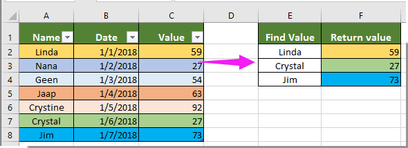
Suponga que tiene una tabla como la que se muestra en la siguiente captura de pantalla. Ahora desea comprobar si un valor especificado está en la columna A y, en ese caso, devolver el valor correspondiente junto con su color de fondo en la columna C. ¿Cómo puede lograrlo? El método descrito en este artículo le ayudará a resolver este problema.
BUSCARV y devolver Color de fondo junto con el valor buscado mediante una función definida por el usuario
Siga los pasos siguientes para buscar un valor y obtener su valor correspondiente junto con el color de fondo en Excel.
1. En la hoja de cálculo que contiene el valor que desea buscar con BUSCARV, haga clic con el botón derecho en la pestaña de la hoja y seleccione Ver código en el menú contextual. Vea la captura de pantalla:

2. En la ventana de Microsoft Visual Basic para Aplicaciones que se abre, copie el siguiente código VBA en la ventana de código.
Código VBA 1: BUSCARV y devolver Color de fondo junto con el valor buscado
Sub Worksheet_Change(ByVal Target As Range)
    Dim I As Long
    Dim xKeys As Long
    Dim xDicStr As String
    On Error Resume Next
    Application.ScreenUpdating = False
    xKeys = UBound(xDic.Keys)
    If xKeys >= 0 Then
        For I = 0 To UBound(xDic.Keys)
            xDicStr = xDic.Items(I)
            If xDicStr <> "" Then
                Range(xDic.Keys(I)).Interior.Color = _
                Range(xDic.Items(I)).Interior.Color
            Else
                Range(xDic.Keys(I)).Interior.Color = xlNone
            End If
        Next
        Set xDic = Nothing
    End If
    Application.ScreenUpdating = True
End Sub
3. A continuación, haga clic en Insertar > Módulo y copie el siguiente código VBA 2 en la ventana del módulo.
Código VBA 2: BUSCARV y devolver Color de fondo junto con el valor buscado
Public xDic As New Dictionary
Function LookupKeepColor (ByRef FndValue, ByRef LookupRng As Range, ByRef xCol As Long)
    Dim xFindCell As Range
    On Error Resume Next
    Set xFindCell = LookupRng.Find(FndValue, , xlValues, xlWhole)
    If xFindCell Is Nothing Then
        LookupKeepColor = ""
        xDic.Add Application.Caller.Address, ""
    Else
        LookupKeepColor = xFindCell.Offset(0, xCol - 1).Value
        xDic.Add Application.Caller.Address, xFindCell.Offset(0, xCol - 1).Address
    End If
End Function
4. Tras insertar ambos códigos, haga clic en Herramientas > Referencias. A continuación, active la casilla Microsoft Script Runtime en el cuadro de diálogo Referencias: VBAProject. Vea la captura de pantalla:

5. Pulse las teclas Alt + Q para cerrar la ventana de Microsoft Visual Basic para Aplicaciones y volver a la hoja de cálculo.
6. Seleccione una celda vacía adyacente al valor buscado, introduzca la fórmula =LookupKeepColor(E2,$A$1:$C$8,3) en la Barra de fórmulas y pulse Intro.

Nota: En la fórmula, E2 contiene el valor que desea buscar, $A$1:$C$8 es el rango de la tabla y el número 3 indica que el valor correspondiente que se devolverá se encuentra en la tercera columna de la tabla. Adáptelos a sus necesidades.
7. Mantenga seleccionada la primera celda de resultados y arrastre el controlador de relleno hacia abajo para obtener todos los resultados con su color de fondo. Vea la captura de pantalla.

Artículos relacionados:
- ¿Cómo se copia el formato de la celda de origen al utilizar BUSCARV en Excel?
- ¿Cómo usar BUSCARV para devolver un formato de fecha en lugar de un número en Excel?
- ¿Cómo se utilizan BUSCARV y SUMA en Excel?
- ¿Cómo usar BUSCARV para obtener el valor de la celda adyacente o siguiente en Excel?
- ¿Cómo buscar un valor con BUSCARV y obtener como resultado VERDADERO o FALSO, o bien SÍ o NO, en Excel?
Las mejores herramientas de productividad para Office
Potencie sus habilidades en Excel con Kutools para Excel y experimente una eficiencia como nunca antes.Kutools para Excel ofrece más de 300 funciones avanzadas para aumentar su productividad y Ahorrar tiempo.Haga clic aquí para obtener la función que más necesita...
Office Tab aporta una interfaz con pestañas a Office y hace que su trabajo sea mucho más fácil
- Active la edición y lectura con pestañas en Word, Excel, PowerPoint, Publisher, Access, Visio y Project.
- Abra y cree varios documentos en nuevas pestañas dentro de la misma ventana, en lugar de hacerlo en ventanas separadas.
- ¡Aumente su productividad en un 50 % y elimine cientos de clics del ratón cada día!
Todos los complementos de Kutools en un solo instalador.
Kutools for Office es la suite que incluye complementos para Excel, Word, Outlook y PowerPoint, además de Office Tab Pro, ideal para equipos que trabajan en distintas aplicaciones de Office.
- Suite integral— complementos para Excel, Word, Outlook y PowerPoint + Office Tab Pro
- Un instalador, una licencia— configuración en minutos (compatible con MSI)
- Rendimiento mejorado en conjunto— productividad optimizada en todas las aplicaciones de Office
- Prueba gratuita de 30 días con todas las funciones— sin registro ni tarjeta de crédito
- La mejor relación calidad-precio— ahorre frente a la compra individual de complementos