Saltar al contenido principal

¿Cómo devolver múltiples valores coincidentes según uno o varios criterios en Excel?

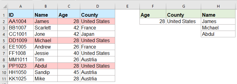
Normalmente, buscar un valor específico y devolver el elemento coincidente es fácil para la mayoría de nosotros usando la función BUSCARV. Pero, ¿alguna vez ha intentado devolver varios valores coincidentes en función de uno o más criterios como se muestra en la siguiente captura de pantalla? En este artículo, presentaré algunas fórmulas para resolver esta compleja tarea en Excel.

Devuelve varios valores coincidentes según uno o varios criterios con fórmulas de matriz


Devuelve varios valores coincidentes según uno o varios criterios con fórmulas de matriz

Por ejemplo, quiero extraer todos los nombres cuya edad sea 28 y provengan de Estados Unidos, por favor aplique la siguiente fórmula:

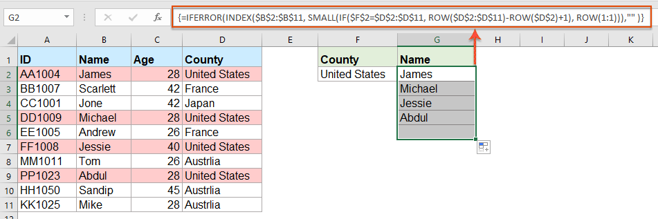
1. Copie o ingrese la fórmula a continuación en una celda en blanco donde desea ubicar el resultado:

=INDEX($B$2:$B$11, SMALL(IF(COUNTIF($F$2, $C$2:$C$11)*COUNTIF($G$2, $D$2:$D$11), ROW($A$2:$D$11)-MIN(ROW($A$2:$D$11))+1), ROW(A1)), COLUMN(A1))

Note: En la fórmula anterior, B2: B11 es la columna de la que se devuelve el valor coincidente; F2, C2: C11 son la primera condición y los datos de la columna que contienen la primera condición; G2, D2: D11 son la segunda condición y los datos de la columna que contienen esta condición, cámbielos según sus necesidades.

2. Entonces presione Ctrl + Shift + Enter claves para obtener el primer resultado coincidente, y luego seleccione la primera celda de fórmula y arrastre el controlador de relleno hacia las celdas hasta que se muestre el valor de error, ahora, todos los valores coincidentes se devuelven como se muestra a continuación en la captura de pantalla:

Tips: Si solo necesita devolver todos los valores coincidentes en función de una condición, aplique la siguiente fórmula de matriz:

=IFERROR(INDEX($B$2:$B$11, SMALL(IF($F$2=$D$2:$D$11, ROW($D$2:$D$11)-ROW($D$2)+1), ROW(1:1))),"" )


Artículos más relativos:

  • Devolver varios valores de búsqueda en una celda separada por comas
  • En Excel, podemos aplicar la función BUSCARV para devolver el primer valor coincidente de las celdas de una tabla, pero, a veces, necesitamos extraer todos los valores coincidentes y luego separarlos por un delimitador específico, como una coma, un guión, etc ... en un solo celda como se muestra en la siguiente captura de pantalla. ¿Cómo podríamos obtener y devolver múltiples valores de búsqueda en una celda separada por comas en Excel?
  • Vlookup y devuelve múltiples valores coincidentes a la vez en la hoja de Google
  • La función normal de Vlookup en la hoja de Google puede ayudarlo a encontrar y devolver el primer valor coincidente basado en un dato dado. Pero, a veces, es posible que deba realizar una búsqueda virtual y devolver todos los valores coincidentes como se muestra en la siguiente captura de pantalla. ¿Tiene alguna forma buena y fácil de resolver esta tarea en la hoja de Google?
  • Vlookup y devuelve varios valores de la lista desplegable
  • En Excel, ¿cómo podría visualizar y devolver múltiples valores correspondientes de una lista desplegable, lo que significa que cuando elige un elemento de la lista desplegable, todos sus valores relativos se muestran a la vez como se muestra en la siguiente captura de pantalla? En este artículo, presentaré la solución paso a paso.
  • Vlookup y devuelve múltiples valores verticalmente en Excel
  • Normalmente, puede usar la función Vlookup para obtener el primer valor correspondiente, pero, a veces, desea devolver todos los registros coincidentes según un criterio específico. En este artículo, hablaré sobre cómo visualizar y devolver todos los valores coincidentes verticalmente, horizontalmente o en una sola celda.
  • Vlookup y devuelve datos coincidentes entre dos valores en Excel
  • En Excel, podemos aplicar la función normal de Vlookup para obtener el valor correspondiente basado en un dato dado. Pero, a veces, queremos visualizar y devolver el valor coincidente entre dos valores como se muestra en la siguiente captura de pantalla, ¿cómo podría manejar esta tarea en Excel?


  • Barra de súper fórmula (edite fácilmente varias líneas de texto y fórmulas); Diseño de lectura (leer y editar fácilmente un gran número de celdas); Pegar en rango filtrado...
  • Combinar celdas / filas / columnas y conservación de datos; Contenido de celdas divididas; Combinar filas duplicadas y suma / promedio... Prevenir celdas duplicadas; Comparar rangos...
  • Seleccione Duplicado o Único Filas; Seleccionar filas en blanco (todas las celdas están vacías); Super Find y Fuzzy Find en muchos libros de trabajo; Selección aleatoria ...
  • Copia exacta Varias celdas sin cambiar la referencia de la fórmula; Crear referencias automáticamente a varias hojas; Insertar viñetas, Casillas de verificación y más ...
  • Fórmulas favoritas e insertar rápidamente, Rangos, gráficos e imágenes; Cifrar celdas con contraseña; Crear lista de distribución y enviar correos electrónicos ...
  • Extraer texto, Agregar texto, Eliminar por posición, Quitar espacio; Crear e imprimir subtotales de paginación; Convertir entre contenido de celdas y comentarios...
  • Súper filtro (guardar y aplicar esquemas de filtros a otras hojas); Orden avanzado por mes / semana / día, frecuencia y más; Filtro especial en negrita, cursiva ...
  • Combinar libros y hojas de trabajo; Combinar tablas basadas en columnas clave; Dividir datos en varias hojas; Conversión por lotes de xls, xlsx y PDF...
  • Agrupación de tablas dinámicas por número de semana, día de la semana y más ... Mostrar celdas bloqueadas y desbloqueadas por diferentes colores; Resalte las celdas que tienen fórmula / nombre...
pestaña kte 201905
  • Habilite la edición y lectura con pestañas en Word, Excel, PowerPoint, Publisher, Access, Visio y Project.
  • Abra y cree varios documentos en nuevas pestañas de la misma ventana, en lugar de en nuevas ventanas.
  • ¡Aumenta su productividad en un 50% y reduce cientos de clics del mouse todos los días!
officetab parte inferior


Comments (25)
No ratings yet. Be the first to rate!
This comment was minimized by the moderator on the site
Hi, if there are duplicate values (e.g. two adams), how do i make sure that it only returns 1 adam and not 2?
This comment was minimized by the moderator on the site
Hello, Bobby,
To extract only unique matching values, you should apply the below formula:
After pasting the formula, please press Ctrl + Shift + Enter keys together to get the correct result.
=IFERROR(INDEX($B$2:$B$5, MATCH(0, COUNTIF(H1:$H$1, $B$2:$B$5)+IF($D$2:$D$5<>$G$2, 1, 0)+IF($C$2:$C$5<>$F$2, 1, 0), 0)), "")

Please have a try, hope it can help you!
This comment was minimized by the moderator on the site
Hi,

Thanks for posting these examples.
I'm trying to implement this in my own sheet, but don't get it to work (maybe because I'm using an europe version of excel)?

I want to get the dates of the days that I had my shifts or that I have worked 'some' (>0) hours for a client.

So in I3 is the name and in J3 the month. K3 and L3 are the shifts (1 is worked) and hours (don't know how to set this, should be more than zero)

My expected results are in:
Shifts: I7 and I8
hours: J7

So I worked more than 0 hours for 'person 2' in oktober on 3-10-2022
had shifts for person 2 on '10-10-2022' and 28-10-2022

When I add '=INDEX($B$2:$B$11, SMALL(IF(COUNTIF($F$2, $C$2:$C$11)*COUNTIF($G$2, $D$2:$D$11), ROW($A$2:$D$11)-MIN(ROW($A$2:$D$11))+1), ROW(A1)), COLUMN(A1))' in my excel sheet, it doesn't allow the comma between the different parts of the formula.
So I need to change them to ';'.
But when I try it it always says: '#NAME?'

So can someone help me with this?

Kind regards,

Bas
[img]https://drive.google.com/file/d/1iIPQKuj_PNhqWyWlwJ4IQTqGNEd6B9Hw/view?usp=share_link[/img]
This comment was minimized by the moderator on the site
Hi,

First, thank you for sharing!

Can you please provide a solution to the case below:

I have 3 columns (A: Containing reference information, B: Containing information to be searched, C: Search result)

Image url is provided below

https://ibb.co/VHCd09K

Column A-------------------------Column B------------Column C
File Name-------------------------Name----------------File Name, Document Name, Element Name, Name
Changed Element-----------------Element--------------Changed Element, Element Name, Element ID
Column Location
Document Name
Element Name
Name
Category
Warranty
Slope
Element ID

What I need is to search in column A for any partial match with cell B2 (Name) or B3 (Element) and get the result in one cell,

Thank you, Behzad
This comment was minimized by the moderator on the site
Hello, Behzad
Maybe the below User Defined Function can help you.
Public Function ConcatPartLookUp(rngInput As Range, rngSource As Range, Optional strDelimiter As String, Optional blCaseSensitive)
Dim rng As Range
If strDelimiter = "" Then strDelimiter = ","
If IsMissing(blCaseSensitive) Then
    blCaseSensitive = False
Else
    blCaseSensitive = True
End If
For Each rng In rngSource
    If blCaseSensitive Then
        If InStr(1, rng.Value, rngInput.Value, vbBinaryCompare) > 0 Then ConcatPartLookUp = ConcatPartLookUp & strDelimiter & rng.Value
    Else
        If InStr(1, rng.Value, rngInput.Value, vbTextCompare) > 0 Then ConcatPartLookUp = ConcatPartLookUp & strDelimiter & rng.Value
    End If
Next
If Len(ConcatPartLookUp) > 0 Then ConcatPartLookUp = Mid(ConcatPartLookUp, 2, Len(ConcatPartLookUp))
End Function


After copying and pasting this code, and then use this formula:=ConcatPartLookUp(B2,$A$2:$A$8) to get the result you need.
Please have a try, hope it can help you!
This comment was minimized by the moderator on the site
Heyi, thank you for the formula. It worked for "fixed" values / text as criterias. However, one of the criterias i'm trying to use is a condition (values <>0 ), but does not work the described formula. Do you guys know what should i change to adapt the formula so I can have a condition as one of the criterias, please?

Best,

João
This comment was minimized by the moderator on the site
Hello, Marcus
To solve your problem, please view this article:
https://www.extendoffice.com/documents/excel/6393-excel-vlookup-function.html#b3-2
There are some detailed explanations of this task. You just need to change the criteira to your own.
Thank you!
This comment was minimized by the moderator on the site
Hi,

if in cell H1 i write "Name" and wanted to link that with the formula, how would that work?
Then I could write "ID" in cell H1 and would automatically get as a result: AA1004; DD1009; PP1023 (for the first formula)

Thank you in advance!
This comment was minimized by the moderator on the site
Hello, Marie
Sorry, i can't get the point of your first problem, could you explain your problem more clearly and detailedly? Or you can insert a screenshot here to describe your problem.
As for the second question, you just need to change the cell reference as this:
=INDEX($A$2:$A$11, SMALL(IF(COUNTIF($F$2, $C$2:$C$11)*COUNTIF($G$2, $D$2:$D$11), ROW($A$2:$D$11)-MIN(ROW($A$2:$D$11))+1), ROW(A1)), COLUMN(A1))

Remeber to press Ctrl + Shift + Enter keys together.
Please try, hope it can help you!
This comment was minimized by the moderator on the site
Hello,
what would be needed to expand the first formula in the following case:
Some IDs are Blank (e.g. cell A5 is blank) and I would like an additional condition outputting lines only when the IDs are not blank. (So the output should then be James and Abdul.
Thanks!
This comment was minimized by the moderator on the site
Hello, Jo,
To solve your problem, please apply the below formula:
=INDEX($B$2:$B$11, SMALL(IF(COUNTIF($F$2, $C$2:$C$11)*COUNTIF($G$2, $D$2:$D$11)*($A$2:$A$11<>0), ROW($A$2:$D$11)-MIN(ROW($A$2:$D$11))+1), ROW(A1)), COLUMN(A1))

Please have a ry, hope it can help you!
This comment was minimized by the moderator on the site
hello,
ive tried using the formula and it either generates a value of 0 or the image attached
This comment was minimized by the moderator on the site
Hello, Milku
Your screenshot showed WPS software of MAC version, so I am not sure whether our formula is available.
I uploaded an Excel file to here, you can try to see if it can calculate correctly in you environment.
Thank you!
This comment was minimized by the moderator on the site
When I use the second formula and drag down, nothing appears. The formula result (fx) says it should be returning something but it is blank. How do I correct this?
This comment was minimized by the moderator on the site
Hello Alysia,

Glad to help. I tried the second formula in the article and drag the formula down, the rest of results were returned. I think there may be two reasons for your problem. First, maybe you forget to press Ctrl + Shift + Enter keys to enter the formula. Second, the matching result is only one, so no other results are not returned. Please have a check.

Sincerely,
Mandy
This comment was minimized by the moderator on the site
Hi,

I was wondering if it at all possible to enter a 2nd criteria but from the same range as the 1st criteria,

For example with the used example above i would like to search for the names of people from both America and France So cell F3 would have France, Scarlett & Andrew would also populate in the list in Column G

Thank you for assistance in advance.
This comment was minimized by the moderator on the site
Hello Nick,

Glad to help. If you want to get the names of people from both America and France, I advise you to use our formula twice to get the result. Please see the screenshot, In F2 and G2 are values "United States" and "France". Apply formula =IFERROR(INDEX($B$2:$B$11, SMALL(IF($F$2=$D$2:$D$11, ROW($D$2:$D$11)-ROW($D$2)+1), ROW(1:1))),"" ) to get the results for America. And apply formula =IFERROR(INDEX($B$2:$B$11, SMALL(IF($G$2=$D$2:$D$11, ROW($D$2:$D$11)-ROW($D$2)+1), ROW(1:1))),"" ) to get the results for France. It's simple. Please have a try.

Sincerely,
Mandy
This comment was minimized by the moderator on the site
In the first example, what change to the formula would be needed to return everyone who was less than 28 years old?
There are no comments posted here yet
Load More
Please leave your comments in English
Posting as Guest
×
Rate this post:
0   Characters
Suggested Locations