¿Cómo cambiar el color de fondo o el color de fuente en función del valor de la celda en Excel?
Al trabajar con grandes volúmenes de datos en Excel, es posible que quieras resaltar ciertos valores aplicando un color de fondo o de fuente específico. Este artículo explica cómo cambiar rápidamente el color de fondo o de fuente según los valores de las celdas en Excel.
Método 1: Cambiar el fondo o el Color de fuente según el valor de la celda de forma dinámica con Usar formato condicional
La función Usar formato condicional le permite resaltar los valores mayores que x, menores que y o comprendidos entre x e y.
Supongamos que tiene un rango de datos y desea resaltar los valores comprendidos entre 80 y 100. Siga estos pasos:
1. Seleccione el rango de celdas en el que quiera resaltar determinadas celdas y, a continuación, haga clic en Inicio > Usar formato condicional > Nueva regla. Consulte la captura de pantalla:

2. En el cuadro de diálogo Nueva regla de formato, seleccione la opción Aplicar formato únicamente a las celdas que contengan en el cuadro Seleccione un tipo de regla y, en la sección Aplicar formato únicamente a las celdas con, especifique las condiciones que necesite:
- En el primer cuadro desplegable, seleccione Valor de celda;
- En el segundo cuadro desplegable, seleccione el criterio:entre;
- En el tercer y cuarto cuadro, introduzca las condiciones de filtro, por ejemplo, 80 y 100.

3. A continuación, haga clic en el botón Formato. En el cuadro de diálogo Establecer formato de celda, configure el fondo o el color de fuente como se muestra a continuación:
| Cambie el Color de fondo según el valor de la celda: | Cambie el Color de fuente según el valor de la celda |
| Haga clic en la pestaña Rellenoy elija uno de los Color de fondo que desee | Haga clic en la pestaña Fuentey seleccione el Color de fuente que necesite. |
 |  |
4. Tras seleccionar el fondo o el color de fuente, haga clic en Aceptar > Aceptar para cerrar los cuadros de diálogo. Ahora, las celdas específicas con valores comprendidos entre 80 y 100 habrán cambiado al fondo o al color de fuente indicado en la selección. Consulte la captura de pantalla:
| Resalte celdas específicas con Color de fondo: | Resalte celdas específicas con Color de fuente: |
 |  |
Nota: La función Usar formato condicional es dinámica; el color de la celda cambiará a medida que se modifiquen los datos.
Método 2: Cambiar el fondo o el Color de fuente según el valor de la celda de forma estática con la función Buscar
A veces, necesitas aplicar un relleno o un color de fuente específico en función del valor de la celda, y que dicho relleno o color de fuente no cambie aunque se modifique el valor de la celda. En ese caso, puedes utilizar la función Buscar para localizar todos los valores de celda específicos y, a continuación, ajustar el color de fondo o de fuente según tus necesidades.
Por ejemplo, si desea cambiar el fondo o el Color de fuente cuando el valor de la celda contenga el texto “Excel”, siga estos pasos:
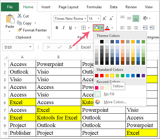
1. Seleccione el rango de datos que desee utilizar y, a continuación, haga clic en Inicio > Buscar y seleccionar > Buscar. Consulte la captura de pantalla:

2. En el cuadro de diálogo Buscar y reemplazar, en la pestaña Buscar, introduzca el valor que desee buscar en el cuadro de texto Buscar qué. Consulte la captura de pantalla:

3. A continuación, haga clic en el botón Buscar todo. En el cuadro de resultados de la búsqueda, haga clic en cualquier elemento y pulse Ctrl + A para seleccionar todos los elementos encontrados. Consulte la captura de pantalla:

4. Por último, haga clic en el botón Cerrar para cerrar este cuadro de diálogo. Ahora ya puede aplicar un fondo o un color de fuente a estos valores seleccionados; consulte la captura de pantalla:
| Aplique el Color de fondo a las celdas seleccionadas: | Aplique el Color de fuente a las celdas seleccionadas: |
 |  |
Método 3: Cambiar el fondo o el Color de fuente según el valor de la celda de forma estática con Kutools para Excel
Kutools para Excel’s Búsqueda avanzada admite numerosas condiciones para buscar valores, cadenas de texto, fechas, fórmulas, celdas con formato, etc. Tras encontrar y seleccionar las celdas coincidentes, puede cambiar el color de fondo o el color de fuente según lo desee.
1. Seleccione el rango de datos que desee buscar y, a continuación, haga clic en Kutools > Búsqueda avanzada. Consulte la captura de pantalla:

2. En el panel Búsqueda avanzada, realice las siguientes operaciones:
- (1.) En primer lugar, haga clic en el icono de la opción Valores;
- (2.) Elija el ámbito de búsqueda en el menú desplegable Dentro de, en este caso, elegiré Selección;
- (3.) En la lista desplegable Tipo, seleccione el criterio que desee utilizar;
- (4.) A continuación, haga clic en el botón Buscarpara mostrar todos los resultados correspondientes en el cuadro de lista;
- (5.) Por último, haga clic en el botón Seleccionar para seleccionar las celdas.

3. A continuación, todas las celdas que coincidan con los criterios se seleccionarán de inmediato. Consulte la captura de pantalla:

4. Ahora puede cambiar el color de fondo o el color de fuente de las celdas seleccionadas según sus necesidades.
Consejos:Con la función Búsqueda avanzada, también puede realizar rápidamente y con facilidad las siguientes operaciones:
Las mejores herramientas de productividad para Office
Potencie sus habilidades en Excel con Kutools para Excel y experimente una eficiencia como nunca antes.Kutools para Excel ofrece más de 300 funciones avanzadas para aumentar su productividad y Ahorrar tiempo.Haga clic aquí para obtener la función que más necesita...
Office Tab aporta una interfaz con pestañas a Office y hace que su trabajo sea mucho más fácil
- Active la edición y lectura con pestañas en Word, Excel, PowerPoint, Publisher, Access, Visio y Project.
- Abra y cree varios documentos en nuevas pestañas dentro de la misma ventana, en lugar de hacerlo en ventanas separadas.
- ¡Aumente su productividad en un 50 % y elimine cientos de clics del ratón cada día!
Todos los complementos de Kutools en un solo instalador.
Kutools for Office es la suite que incluye complementos para Excel, Word, Outlook y PowerPoint, además de Office Tab Pro, ideal para equipos que trabajan en distintas aplicaciones de Office.
- Suite integral— complementos para Excel, Word, Outlook y PowerPoint + Office Tab Pro
- Un instalador, una licencia— configuración en minutos (compatible con MSI)
- Rendimiento mejorado en conjunto— productividad optimizada en todas las aplicaciones de Office
- Prueba gratuita de 30 días con todas las funciones— sin registro ni tarjeta de crédito
- La mejor relación calidad-precio— ahorre frente a la compra individual de complementos