Resaltado automático de la fila y columna activa en Excel (Guía completa)
Navegar por extensas hojas de cálculo de Excel llenas de datos puede ser un desafío, y es fácil perder de vista tu posición o malinterpretar valores. Para mejorar tu análisis de datos y reducir el riesgo de errores, presentaremos 3 formas diferentes de resaltar dinámicamente la fila y columna de una celda seleccionada en Excel. A medida que te mueves de celda a celda, el resaltado cambia dinámicamente, proporcionando una pista visual clara e intuitiva para mantenerte enfocado en los datos correctos, como se muestra en la siguiente demostración:
Resaltado automático de la fila y columna activa en Excel
- Con código VBA -Limpia el color existente de las celdas, no admite Deshacer
- Solo un clic de Kutools para Excel -Mantiene el color existente de las celdas, admite Deshacer, funciona en hojas protegidas
- Con Formato Condicional -No es estable con grandes volúmenes de datos, requiere actualización manual (F9)
Resaltado automático de la fila y columna activa con código VBA
Para resaltar automáticamente toda la columna y fila de la celda seleccionada en la hoja de trabajo actual, el siguiente código VBA puede ayudarte a lograr esta tarea.
Paso 1: Abre la hoja de trabajo donde deseas resaltar automáticamente la fila y columna activa
Paso 2: Abre el editor del módulo de la hoja VBA y copia el código
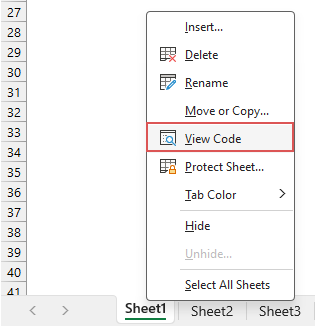
- Haz clic derecho en el nombre de la hoja y elige "Ver Código" desde el menú contextual, ver captura de pantalla:
- En el editor del módulo de la hoja VBA abierto, copia y pega el siguiente código en el módulo en blanco. Ver captura de pantalla:
Código VBA: resalta la fila y columna de la celda seleccionadaPrivate Sub Worksheet_SelectionChange(ByVal Target As Range) 'Update by Extendoffice Dim rowRange As Range Dim colRange As Range Dim activeCell As Range Set activeCell = Target.Cells(1, 1) Set rowRange = Rows(activeCell.Row) Set colRange = Columns(activeCell.Column) Cells.Interior.ColorIndex = xlNone rowRange.Interior.Color = RGB(248, 150, 171) colRange.Interior.Color = RGB(173, 233, 249) End SubConsejos: Personaliza el código- Para cambiar el color de resaltado, simplemente necesitas modificar el valor RGB en los siguientes scripts:
rowRange.Interior.Color = RGB(248, 150, 171)
colRange.Interior.Color = RGB(173, 233, 249) - Para resaltar solo la fila completa de la celda seleccionada, elimina o comenta (agrega un apóstrofe al inicio de) esta línea:
colRange.Interior.Color = RGB(173, 233, 249) - Para resaltar solo la columna completa de la celda seleccionada, elimina o comenta (agrega un apóstrofe al inicio de) esta línea:
rowRange.Interior.Color = RGB(248, 150, 171)

- Para cambiar el color de resaltado, simplemente necesitas modificar el valor RGB en los siguientes scripts:
- Luego, cierra la ventana del editor VBA para regresar a la hoja de trabajo.


Resultado:
Ahora, cuando selecciones una celda, la fila y columna completas de esa celda se resaltan automáticamente, y el resaltado cambia dinámicamente a medida que cambia la celda seleccionada, como se muestra en la siguiente demostración:
- Este código borrará los colores de fondo de todas las celdas en la hoja de trabajo, así que evita usar esta solución si tienes celdas con colores personalizados.
- Ejecutar este código deshabilitará la función "Deshacer" en la hoja, lo que significa que no podrás revertir errores presionando el atajo "Ctrl" + "Z".
- Este código no funcionará en una hoja de trabajo protegida.
- Para detener el resaltado de la fila y columna de la celda seleccionada, deberás eliminar el código VBA previamente agregado. Después de eso, para restablecer el resaltado haz clic en "Inicio" > "Color de relleno" > "Sin relleno".
Resaltado automático de la fila y columna activa con un solo clic de Kutools
¿Enfrentando limitaciones del código VBA en Excel? ¡La función "Cuadrícula de enfoque" de "Kutools para Excel" es tu solución ideal! Diseñada para abordar las deficiencias del VBA, ofrece una amplia gama de estilos de resaltado para mejorar tu experiencia en la hoja. Con su capacidad para aplicar estos estilos en todos los libros abiertos, "Kutools" garantiza un proceso de gestión de datos eficiente y visualmente atractivo.
Después de instalar Kutools para Excel, haz clic en "Kutools" > "Cuadrícula de enfoque" para habilitar esta función. Ahora puedes ver que la fila y columna de la celda activa se resaltan inmediatamente. Este resaltado cambia dinámicamente mientras cambias la selección de celdas. Ver la demostración a continuación:
- Preserva los colores de fondo originales de las celdas:
A diferencia del código VBA, esta función respeta el formato existente de tu hoja de trabajo. - Utilizable en hojas protegidas:
Esta función funciona sin problemas dentro de hojas protegidas, lo que la hace ideal para gestionar documentos sensibles o compartidos sin comprometer la seguridad. - No afecta la función Deshacer:
Con esta función, conservas acceso completo a la funcionalidad de deshacer de Excel. Esto asegura que puedas revertir cambios fácilmente, añadiendo una capa de seguridad a tu manipulación de datos. - Rendimiento estable con grandes volúmenes de datos:
Esta función está diseñada para manejar grandes conjuntos de datos de manera eficiente, asegurando un rendimiento estable incluso en hojas complejas e intensivas en datos. - Múltiples estilos de resaltado:
Esta función ofrece una variedad de opciones de resaltado, permitiéndote elegir entre diferentes estilos y colores para hacer que tu celda activa de fila, columna o ambas destaque de la manera que mejor se adapte a tus preferencias y necesidades.

- Para desactivar esta función, haz clic en "Kutools" > "Cuadrícula de enfoque" nuevamente para cerrar esta función;
- Para aplicar esta función, descarga e instala Kutools para Excel.
Resaltado automático de la fila y columna activa con Formato Condicional
En Excel, también puedes configurar Formato Condicional para resaltar automáticamente la fila y columna activa. Para configurar esta función, sigue estos pasos:
Paso 1: Selecciona el rango de datos
Primero, selecciona el rango de celdas al que deseas aplicar esta función. Puede ser toda la hoja de trabajo o un conjunto de datos específico. Aquí, seleccionaré toda la hoja de trabajo.
Paso 2: Accede al Formato Condicional
Haz clic en "Inicio" > "Formato condicional" > "Nueva regla", ver captura de pantalla:
Paso 3: Configura las operaciones en la Nueva Regla de Formato
- En el cuadro de diálogo "Nueva Regla de Formato", elige "Usar una fórmula para determinar qué celdas formatear" desde la lista "Seleccionar un tipo de regla".
- En el cuadro "Formatear valores donde esta fórmula es verdadera", ingresa una de estas fórmulas; en este ejemplo, aplicaré la tercera fórmula para resaltar la fila y columna activa.
Para resaltar la fila activa:
Para resaltar la columna activa:=CELL("row")=ROW()
Para resaltar la fila y columna activa:=CELL("col")=COLUMN()=OR(CELL("row")=ROW(), CELL("col")= COLUMN()) - Luego, haz clic en el botón "Formato".

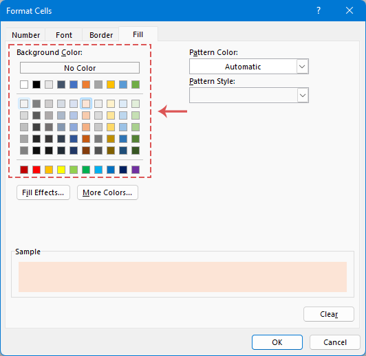
- En el cuadro de diálogo "Formato de celdas" que aparece, bajo la pestaña "Relleno", elige un color para resaltar la fila y columna activa según sea necesario, ver captura de pantalla:
- Luego, haz clic en "Aceptar" > "Aceptar" para cerrar los cuadros de diálogo.


Resultado:
Ahora puedes ver que toda la columna y fila de la celda A1 han sido resaltadas de inmediato. Para aplicar este resaltado a otra celda, simplemente haz clic en la celda deseada y presiona la tecla "F9" para actualizar la hoja, lo que luego resaltará toda la columna y fila de la nueva celda seleccionada.
- De hecho, aunque el enfoque de Formato Condicional para resaltar en Excel ofrece una solución, no es tan fluido como usar "VBA" y la función "Cuadrícula de enfoque". Este método requiere recalcular manualmente la hoja (presionando la tecla "F9").
Para habilitar el recálculo automático de tu hoja de trabajo, puedes incorporar un simple código VBA en el módulo de código de tu hoja objetivo. Esto automatizará el proceso de actualización, asegurando que el resaltado se actualice inmediatamente al seleccionar diferentes celdas sin presionar la tecla "F9". Haz clic derecho en el nombre de la hoja y luego elige "Ver Código" desde el menú contextual. Luego copia y pega el siguiente código en el módulo de la hoja:Private Sub Worksheet_SelectionChange(ByVal Target As Range) Target.Calculate End Sub - El Formato Condicional preserva el formato existente que has aplicado manualmente a tu hoja de trabajo.
- Se sabe que el Formato Condicional es volátil, especialmente cuando se aplica a conjuntos de datos muy grandes. Su uso extensivo puede potencialmente ralentizar el rendimiento de tu libro, afectando la eficiencia del procesamiento y navegación de datos.
- La función CELDA solo está disponible en versiones de Excel 2007 y posteriores, este método no es compatible con versiones anteriores de Excel.
Comparación de los métodos anteriores
| Característica | Código VBA | Formato Condicional | Kutools para Excel |
| Preservar el color de fondo de la celda | No | Sí | Sí |
| Admite Deshacer | No | Sí | Sí |
| Estable en grandes conjuntos de datos | No | No | Sí |
| Utilizable en hojas protegidas | No | Sí | Sí |
| Se aplica a todos los libros abiertos | Solo hoja actual | Solo hoja actual | Todos los libros abiertos |
| Requiere actualización manual (F9) | No | Sí | No |
Eso concluye nuestra guía sobre cómo resaltar la columna y fila de una celda seleccionada en Excel. Si estás interesado en explorar más consejos y trucos de Excel, nuestro sitio web ofrece miles de tutoriales, haz clic aquí para acceder a ellos. ¡Gracias por leer, y esperamos proporcionarte más información útil en el futuro!
Artículos relacionados:
- Resaltado automático de la fila y columna de la celda activa
- Cuando ves una hoja de trabajo grande con numerosos datos, es posible que quieras resaltar la fila y columna de la celda seleccionada para poder leer los datos fácil e intuitivamente y evitar malentendidos. Aquí, puedo presentarte algunos trucos interesantes para resaltar la fila y columna de la celda actual; cuando cambia la celda, la columna y fila de la nueva celda se resaltan automáticamente.
- Resaltar cada otra fila o columna en Excel
- En una hoja de trabajo grande, resaltar o rellenar cada otra fila o columna mejora la visibilidad y legibilidad de los datos. No solo hace que la hoja de trabajo se vea más ordenada, sino que también te ayuda a comprender los datos más rápido. En este artículo, te guiaremos a través de varios métodos para sombrear cada otra fila o columna, ayudándote a presentar tus datos de una manera más atractiva y sencilla.
- Resaltar toda la fila mientras se desplaza
- Si tienes una hoja de trabajo grande con múltiples columnas, será difícil distinguir los datos en esa fila. En este caso, puedes resaltar toda la fila de la celda activa para que puedas ver rápidamente y fácilmente los datos en esa fila cuando desplaces la barra de desplazamiento horizontal. Este artículo hablará sobre algunos trucos para resolver este problema.
- Resaltar filas basadas en una lista desplegable
- Este artículo hablará sobre cómo resaltar filas basadas en una lista desplegable, tomando la siguiente captura de pantalla como ejemplo: cuando selecciono “En progreso” de la lista desplegable en la columna E, necesito resaltar esa fila con color rojo; cuando selecciono “Completado” de la lista desplegable, necesito resaltar esa fila con color azul, y cuando selecciono “No iniciado”, un color verde se usará para resaltar la fila.
Las mejores herramientas de productividad para Office
Mejora tu dominio de Excel con Kutools para Excel y experimenta una eficiencia sin precedentes. Kutools para Excel ofrece más de300 funciones avanzadas para aumentar la productividad y ahorrar tiempo. Haz clic aquí para obtener la función que más necesitas...
Office Tab incorpora la interfaz de pestañas en Office y facilita mucho tu trabajo
- Habilita la edición y lectura con pestañas en Word, Excel, PowerPoint, Publisher, Access, Visio y Project.
- Abre y crea varios documentos en nuevas pestañas de la misma ventana, en lugar de hacerlo en ventanas separadas.
- ¡Aumenta tu productividad en un50% y reduce cientos de clics de ratón cada día!
Todos los complementos de Kutools. Un solo instalador
El paquete Kutools for Office agrupa complementos para Excel, Word, Outlook y PowerPoint junto con Office Tab Pro, ideal para equipos que trabajan en varias aplicaciones de Office.
- Suite todo en uno: complementos para Excel, Word, Outlook y PowerPoint + Office Tab Pro
- Un solo instalador, una licencia: configuración en minutos (compatible con MSI)
- Mejor juntos: productividad optimizada en todas las aplicaciones de Office
- Prueba completa de30 días: sin registro ni tarjeta de crédito
- La mejor relación calidad-precio: ahorra en comparación con la compra individual de complementos